Chapter 7b: Rings, Rulers, and Warps in AAT Space

The previous chapter introduced Codec A, a way to represent a real-valued vector as an AAT. It divides a 128-number vector into 64 slots, with two numbers in each slot. Each pair is replaced by the address of its nearest representative point, or centroid, in a codebook. At six bits per address, a 256-byte vector of 16-bit floats becomes a 48-byte code. Decoding those addresses recovers the vector with roughly 0.98 cosine similarity.

That is a useful representation, but its cost depends on more than the size of the code. Encoding requires a nearest-centroid search in every slot. Computing an inner product directly from two codes requires a table of precomputed products in Codec A, and those tables contain more than a quarter of a million entries. The code is small; the machinery that produces and uses it is much larger.

This chapter develops a more practical design.

What we measure#

A codec must preserve the information its consumer needs. The encode–decode round trip is the first check:

$$\mathbb{R}^{128} \;\xrightarrow{\ \text{encode}\ }\; \mathbb{A}_{64}^{64} \;\xrightarrow{\ \text{decode}\ }\; \mathbb{R}^{128}.$$

Here, $\mathbb{A}_{S}^{k}=\mathbb{A}_{64}^{64}$ is the space of sequences containing 64 symbols, each chosen from an alphabet of 64 possibilities. The superscript $k$ gives the sequence length, and the subscript $S$ gives the alphabet size. Reconstruction cosine measures how closely the decoded vector points in the original direction. It does not measure whether the vector has retained its length. Doubling every coordinate, for example, leaves cosine similarity unchanged while doubling the length and changing every inner product with another vector.

We therefore evaluate three properties: reconstruction direction, recovery of inner products, and recovery of vector lengths. For inner products and lengths, we examine correlation with the original values; length error also measures how far the magnitudes have shifted. Correlation and cosine are useful summaries, but neither alone guarantees that an operation returns the right numerical scale.

The transformer comparisons use activations captured from a middle layer of Qwen3-0.6B, with codebooks fitted on a training split and evaluated on held-out vectors. Unless a different space is specified, the examples use 128-dimensional query vectors with six bits per two-number slot. The lane-input experiment uses 1,024-dimensional vectors; its results are reported separately.

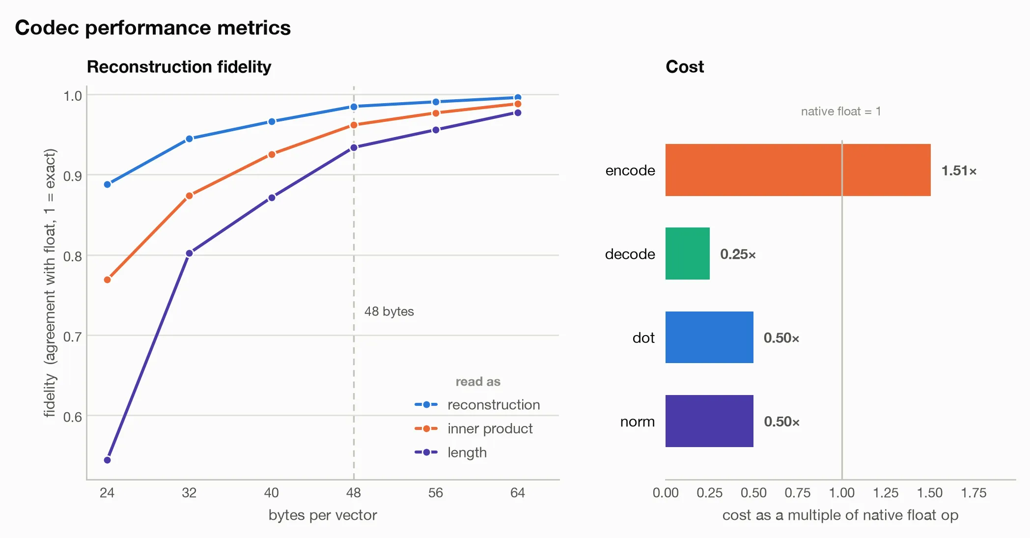
Memory has two separate costs. The first is the number of bytes in each encoded vector. The second is the stored information shared by all vectors: reconstruction values, encoding boundaries, routing information, and any tables used by arithmetic kernels. A codebook stores representative values. A lookup table, or LUT, describes how stored values are accessed. A codebook can be a LUT, but a table of precomputed centroid-to-centroid products is an additional object, often a much larger one.

We also count the work required to encode, decode, and operate on the codes. The benchmark expresses this work in elementary operations, then compares it with the corresponding operation on floating-point vectors.

The cost of a separate codebook for every slot#

Codec A gives each of the 64 slot positions its own codebook. This lets the centroids adapt to the distribution at that position. In this chapter’s query-vector comparison, it reaches 0.991 reconstruction cosine and 0.990 inner-product correlation at six bits per slot. It provides a strong reference for the lower-cost designs.

Its large memory requirement comes from precomputing the arithmetic. With 64 centroids per slot, the table for an inner product needs $64 \times 64$ entries at each of 64 positions:

$$64 \times 64 \times 64 = 262{,}144 \text{ entries}.$$

At two bytes per entry, the product tables occupy 524,288 bytes. Including the reconstruction codebooks brings the total to about 540 KB. At eight bits per slot, the alphabet grows to 256 centroids and the total approaches 8.5 MB. These are shared tables, in addition to the bytes carried by each code.

Encoding has a different scaling problem. The baseline encoder compares each pair with every centroid in its slot. Its counted cost is about 48 native dot products at six bits, rising to 193 at eight bits. Increasing the alphabet improves reconstruction, but makes both the search and the product tables more expensive.

Whether that tradeoff is acceptable depends on how often the code will be reused. PQCache applies product quantization to keys during prefill and uses the codes during later decoding steps to identify important tokens. Repeated use can justify a substantial initial cost. For our lane inputs, however, a new vector must be encoded at each layer for each token. We need to reduce that recurring cost as well as the table size.

Rings: calculate an address from geometry#

To replace the full centroid search, we need a codebook whose addresses are easy to calculate. Since we care about preserving both length and direction, a natural first attempt is to encode those two properties separately.

Codec C, the polar codec, uses stored radii and evenly spaced angles. Their combinations form a grid of rings and spokes. For a slot $x = (x_0, x_1)$:

$$r = \sqrt{x_0^2 + x_1^2}, \qquad \theta = \operatorname{atan2}(x_1, x_0).$$

With $S_\theta$ spokes, dividing the angle by the spoke spacing and rounding gives

$$j = \operatorname{round}\!\left(\frac{S_\theta\theta}{2\pi}\right) \bmod S_\theta.$$

The modulo wraps around the circle. The nearest stored radius gives the ring index $i$; the symbol is $iS_\theta+j$. With $S_r$ stored radii, two scalar assignments replace comparisons with all $S_rS_\theta$ centroids.

That makes encoding cheap: about 0.3 native dot products in the benchmark’s operation model. But reconstruction and length fidelity are too low for our needs. Separating radius and angle has not given us a grid that fits these activation distributions.

The useful result is that separate coordinate assignments make encoding cheap. We now need a grid that also preserves the data well.

Rulers: represent each pair with two scalar quantizers#

Many two-number slots form an elongated cloud along a diagonal. Quantizing the original axes separately spends levels on combinations that the data rarely uses, as Chapter 7 illustrated. A change of coordinates can make a simple grid more effective.

For each pair, form a scaled sum and difference:

$$\begin{pmatrix} u \\ v \end{pmatrix} = H\begin{pmatrix} x_0 \\ x_1 \end{pmatrix}, \qquad H = \frac{1}{\sqrt{2}} \begin{pmatrix} 1 & 1 \\ 1 & -1 \end{pmatrix}.$$

Thus $u=(x_0+x_1)/\sqrt{2}$ and $v=(x_0-x_1)/\sqrt{2}$. When the two original coordinates tend to rise and fall together, the sum describes their common variation and the difference describes how far they diverge. This fixed Hadamard transform aligns its axes with the two diagonals of the original plane. It requires no fitted rotation parameters.

The factor $1/\sqrt{2}$ makes the transform orthogonal: $H^\top H=I$. Lengths, angles, and inner products are preserved before quantization. For two slots $x$ and $y$,

$$\begin{aligned} u_xu_y+v_xv_y &= \frac{(x_0+x_1)(y_0+y_1)+(x_0-x_1)(y_0-y_1)}{2} \\ &= x_0y_0+x_1y_1. \end{aligned}$$

The cross terms cancel. We can therefore work in the sum-and-difference coordinates without changing the underlying dot product.

Codec D quantizes $u$ and $v$ separately. Each axis gets a short list of representative values: a one-dimensional ruler. With eight levels on each axis, the pair has $8 \times 8=64$ possible reconstructions and still fits in a six-bit symbol. If the two level indices are $q_u$ and $q_v$, the symbol is $8q_u+q_v$.

The storage reduction follows from this product structure. We need to store only eight values for $u$ and eight for $v$. At two bytes per value, that is only 32 bytes! To compute a slot’s inner product, retrieve the appropriate values, multiply along each axis, and add the two products.

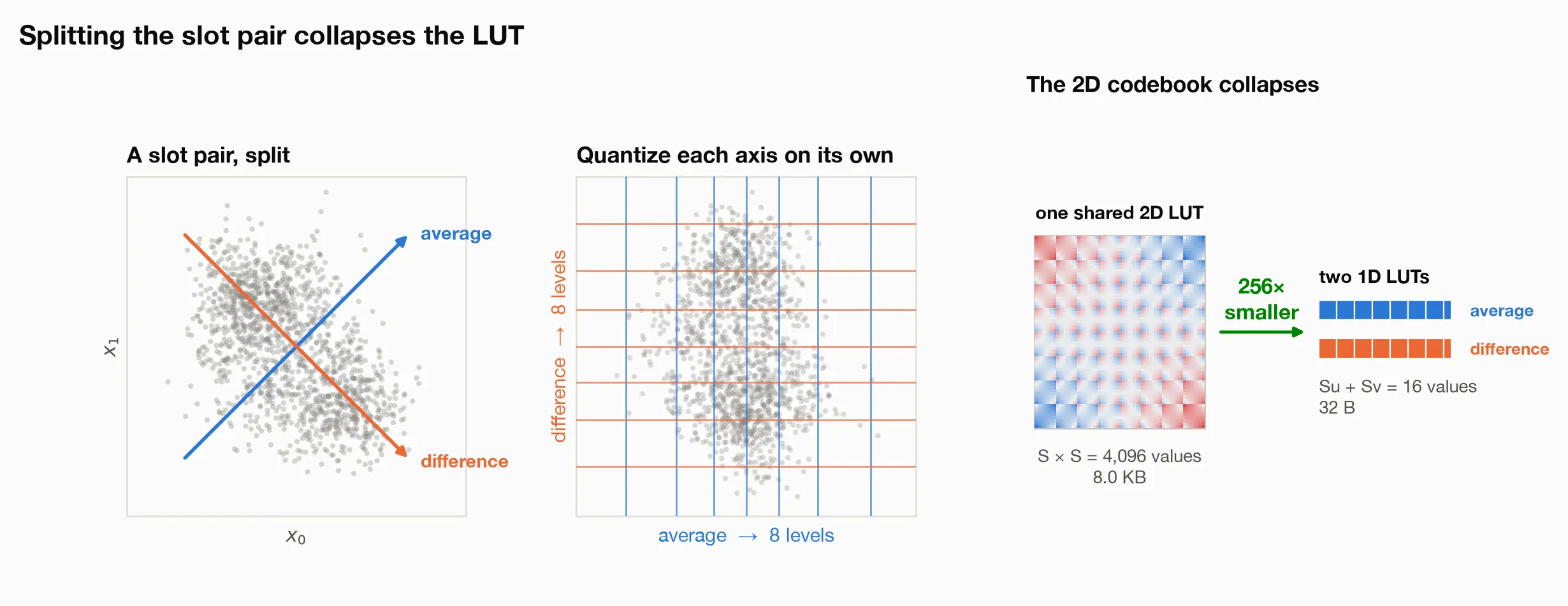
The diagram above compares Codec B’s shared 8 KB product table with Codec D’s 32 bytes of scalar reconstruction values—a 256-fold reduction. Codec B shares one two-dimensional codebook across all slots; Codec A stores a separate codebook and product table at every position, accounting for its roughly half-megabyte total.

At six bits, Codec D reaches 0.965 reconstruction cosine, compared with Codec A’s 0.991. Its fixed diagonal axes need not align with every slot distribution or make the coordinates independent. To test whether fitting the axes helps, Codec E uses principal component analysis (PCA). At six and eight bits, its reconstruction accuracy is similar to Codec D’s, so we retain the simpler fixed Hadamard transform.

Share codebooks among similar slots#

Codec D’s main limitation is that one pair of rulers must serve all 64 positions. The positions do not have the same distribution. Some usually contain small values; others carry much larger values or have a mean far from zero.

To see the difference, write the pair at slot $m$ in training vector $n$ as $a_m^{(n)}$. Its average energy is

$$E_m = \frac{1}{N}\sum_{n=1}^{N}\left\lVert a_m^{(n)}\right\rVert^2.$$

This measures the average squared distance from the origin. A second statistic measures how far the slot’s mean lies from zero:

$$d_m = \left\lVert\frac{1}{N}\sum_{n=1}^{N}a_m^{(n)}\right\rVert.$$

These quantities describe different features. A slot that varies widely and symmetrically around zero can have high energy but almost no mean displacement. A slot concentrated around a nonzero value can have a substantial displacement even if its variation is small.

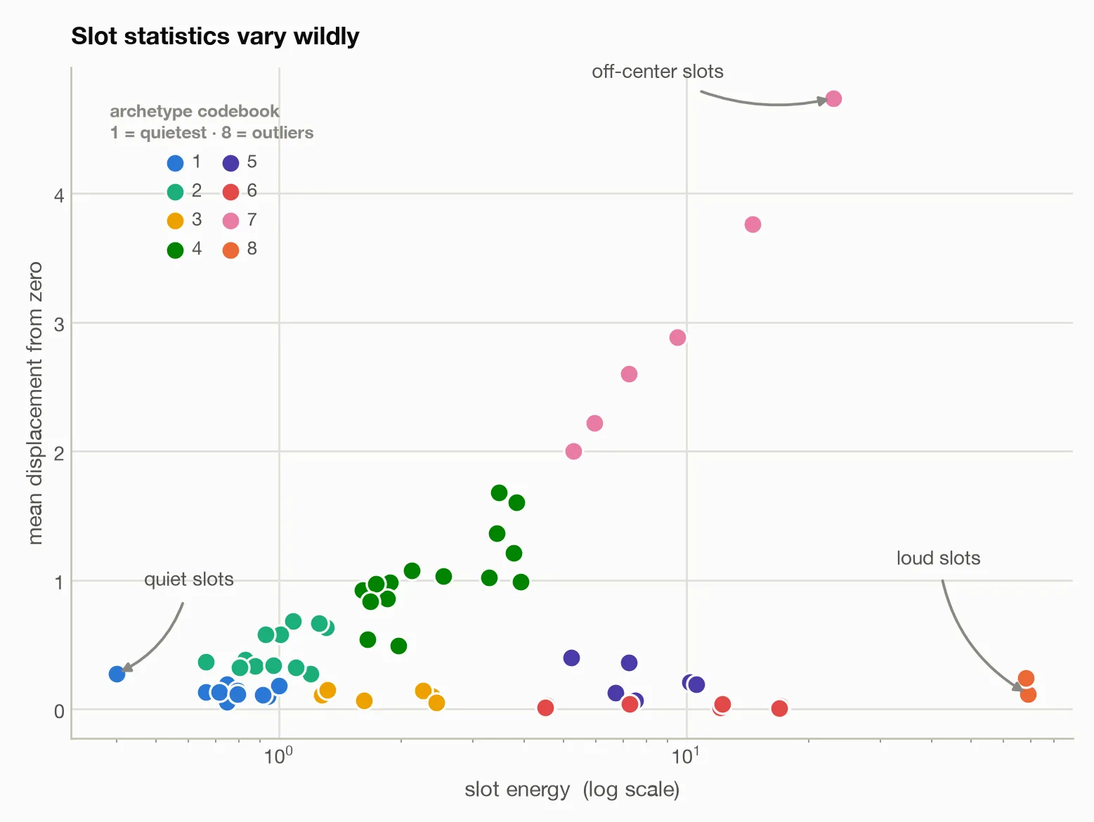
Codec G groups positions by their distribution statistics and fits one separable codebook to each group. We call these groups archetypes. Eight archetypes provide a middle ground between one book shared by every slot and 64 books fitted separately. The grouping also considers tail behavior, beyond the two statistics drawn in the figure.

Each position has a fixed group assignment. Slot 12, for example, always uses the book assigned to slot 12. Both encoder and decoder know the position, so the assignment needs no extra bits in each transmitted code. The small routing table is stored with the codec.

At six bits per slot, Codec G reaches 0.985 reconstruction cosine and 0.966 inner-product correlation, with a reported compact table size of 280 bytes. It recovers much of Codec A’s reconstruction quality while retaining the small scalar codebooks. In the comparison with shared two-dimensional PQ, it improves reconstruction, inner products, and length fidelity with a table about 30 times smaller.

The few-hundred-byte figures describe a compact representation of shared scalar values and routing. A software implementation may expand those values into per-slot codewords or cache additional tables to make particular operations easier. Those expanded buffers occupy more memory. The compact size tells us what must be represented; it does not describe every possible runtime layout.

Warps: place the ruler’s marks from the data#

Small codebooks solve the storage problem, but we still need an efficient encoder. Codec G reduces the search to small one-dimensional codebooks. Codec N goes further by constructing the quantization intervals directly from the distribution of each coordinate.

This matters especially at the input to a neural lane. A transformer’s residual stream is the real-valued vector passed from block to block for each token. Attention and MLP blocks read from it and add their outputs back to it. One practical way to connect lanes to this architecture is to keep the residual stream in real-valued form and encode a fresh AAT wherever a lane needs an input. The cost of that conversion is paid repeatedly.

An effective scalar quantizer uses narrow intervals where values are common and wider intervals where they are rare. Companding gives us a systematic way to choose that spacing. It maps a coordinate through a monotone curve, quantizes the transformed coordinate uniformly, and maps the selected level back to the original units. The curve changes the ruler’s spacing while preserving the order of the values.

Let $p(u)$ be the probability density of one transformed coordinate. The high-resolution approximation assumes that quantization bins are narrow enough for the density to vary little within each bin. Under this approximation, the scalar quantizer that minimizes mean-squared error has a level density proportional to $p(u)^{1/3}$. This is the classical Panter–Dite result; the compander treatment by Jacques, Hammond, and Fadili describes the approximation and its assumptions. Integrating and normalizing this density gives a warp from the coordinate range to $[0,1]$:

$$w(u) = \frac{\displaystyle\int_{-\infty}^{u}p(s)^{1/3}\,ds} {\displaystyle\int_{-\infty}^{+\infty}p(s)^{1/3}\,ds}.$$

Where the data is dense, the curve rises more steeply. Equal intervals on its vertical axis then correspond to smaller intervals in the original coordinate. The cube root balances finer resolution in common regions against the error from representing rare values too coarsely. This spacing minimizes mean-squared error under the narrow-bin approximation; with small alphabets, we still need to check its performance experimentally.

From a fitted curve to stored boundaries#

The encoder does not evaluate those integrals for every input. During fitting, it builds a histogram, takes the cube root of each bin count, forms the cumulative sum, and normalizes it. That produces a numerical approximation to $w$.

For an axis with $S_u$ bins, the encoder stores the $S_u-1$ boundaries

$$b_j = w^{-1}\!\left(\frac{j}{S_u}\right), \qquad j=1,\ldots,S_u-1.$$

With eight bins, these are the seven points where the fitted curve reaches $1/8,2/8,\ldots,7/8$. At runtime, the coordinate is assigned to the interval between its neighboring boundaries. Conceptually, this is a uniform bin assignment in warped space:

$$q_u = \min\!\left(S_u-1,\left\lfloor S_u\,w(u)\right\rfloor\right).$$

The implementation obtains that index from the stored boundaries. It keeps a reconstruction value for each bin, fitted as the mean of the training values assigned there. The same process is applied to $v$, and the two bin indices are packed into one slot symbol. The total alphabet is $S_uS_v$; the bit budget can be divided between the axes according to their variation.

This removes the need to calculate distances to candidate centroids. It also separates two jobs that are easy to confuse: boundaries determine the input’s symbol, while reconstruction values determine what that symbol decodes to.

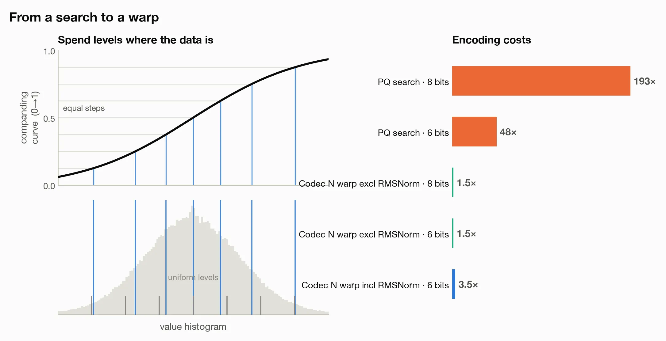
The encoder still has to find which interval contains each coordinate. Searching the ordered boundaries can take more comparisons as the number of bins grows. The benchmark counts this entire assignment as one lookup, giving a flat estimate of about 1.5 native dot products. Actual cost depends on how the search is implemented. The saving is that encoding no longer calculates distances to every centroid.

Codec N was also evaluated on the 1,024-dimensional normalized vectors used as lane inputs. At six bits per slot, 512 slots produce a 384-byte AAT. On those vectors, Codec N reaches 0.984 reconstruction cosine, compared with 0.985 for Codec G. The change in how the bins are fitted costs only 0.001 in this measurement. Codec N additionally stores the encoding boundaries, so its compact tables are larger than Codec G’s reconstruction tables alone.

Accounting for normalization#

In the tested transformer, a block applies RMSNorm before using its residual-stream input. RMSNorm divides the vector by its root-mean-square magnitude, with a small stabilizing constant, then applies a learned gain to each coordinate. The floating-point model already performs this work.

Codec N can include that normalization in its input path: take the residual vector, normalize it, transform each pair, and assign its two bin indices. Counting the whole path gives about 3.5 native dot products. Approximately 2.0× is the normalization already required by the source model, leaving 1.5× as the additional encoding cost under the benchmark’s accounting.

Scalar quantization also appears in image tokenizers. Finite Scalar Quantization, or FSQ, quantizes each coordinate of a small learned representation to a fixed set of values and obtains an implicit codebook from their combinations. Codec N uses a related product structure, with intervals fitted to the activation distribution through companding.

The resulting vector codec#

Each stage of the search contributed to the final design. Rings showed how regular codebooks simplify encoding; rulers reduced storage through separate sum-and-difference quantizers; archetypes let similar slots share their scalar values; warps supplied boundaries fitted to the data. The resulting codec combines the grouping strategy of Codec G with the companding encoder of Codec N.

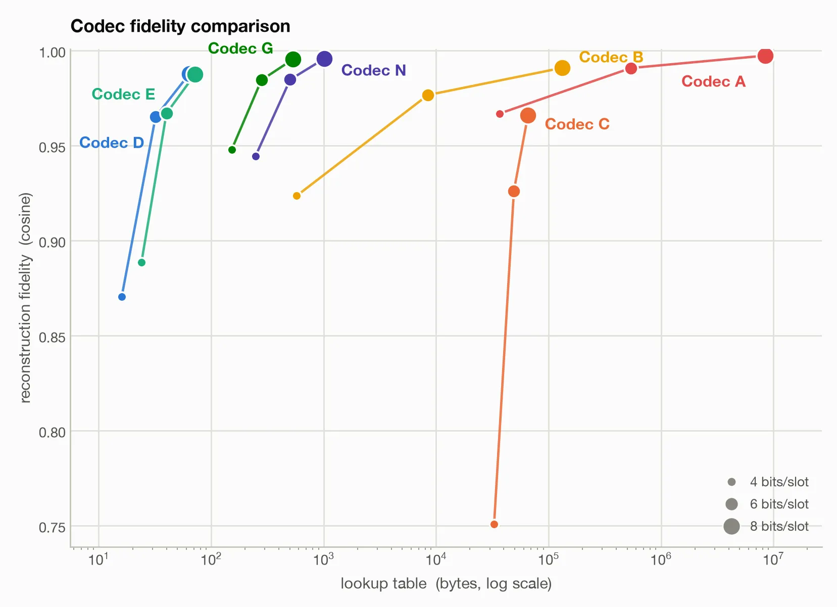
At the illustrated working point, we retain reconstruction cosine near 0.98 with compact tables of a few hundred bytes and scalar bin assignments in place of exhaustive centroid searches. This addresses both costs that motivated the search: shared storage and repeated encoding.

The small reconstruction tables still require arithmetic to compute inner products. Chapter 7c develops attention scores, weighted value sums, and vector norms from the symbols and their stored values.