Chapter 7: The AAT Codec

The iris flowers made encoding easy. Four measurements, four rulers. Each measurement dropped into a bin on its own ruler. Four numbers became a four-symbol AAT.

It worked because the four measurements are genuinely separate. A wide petal tells you nothing about a narrow sepal, so binning each one alone throws almost nothing away.

Most vectors are not like this. A transformer’s vectors have dimensions that move together.

So how do you turn a whole vector into an AAT?

Binning a whole vector#

Start with two numbers so we can draw it: a vector $\mathbf{x} = (x_1, x_2)$ in $\mathbb{R}^2$, one point on a plane. When $x_1$ is large, $x_2$ usually is too, so the points form a diagonal streak.

Bin each axis: eight slices across, eight up, sixty-four cells. The data only visits the cells along the diagonal. You laid out sixty-four cells and used twenty-three, because neither ruler knows what the other is doing.

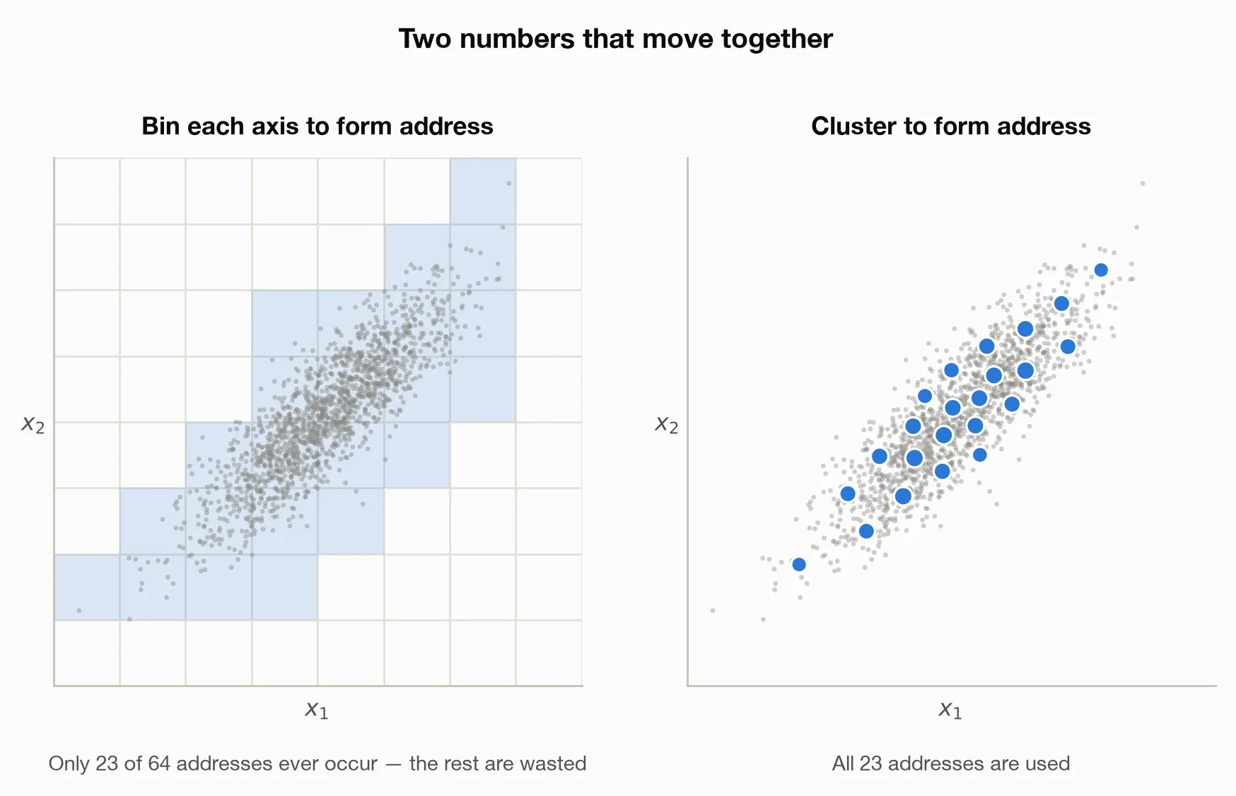
The A2D encoder from the last chapter softened this. Each axis slides its bin edges toward where the data piled up. For four loosely related measurements that is enough. But an adaptive ruler fixes the spacing within an axis, and the diagonal is a fact about two axes at once.

One address for a whole vector?#

The data clumps, so put the addresses on the clumps. Drop a few dozen reference points, called centroids, where the vectors sit. To encode a vector, find its nearest centroid and write down that centroid’s index: “nearest to centroid #37” instead of “bin 3 on $x_1$, bin 5 on $x_2$.”

Finding those clumps is what k-means does. Give it vectors and ask for S clusters. It places S centroids so every vector ends up near one. Replacing a vector with its nearest centroid is vector quantization. It is decades old and runs inside everything from old speech coders to modern audio. Every field that reinvented it renamed the parts. Compression calls the set of centroids a codebook and each entry a codeword. Sparse coding calls it a dictionary of atoms. All of them mean a learned, indexed list of representative vectors. We say centroid, and codebook for the list that holds them.

But there is a problem. To address $\mathbb{R}^{128}$ as finely as we addressed that square, the number of centroids explodes. High-dimensional space is nearly all corners and emptiness, the curse of dimensionality. A centroid near every vector would need a codebook bigger than the model itself. One symbol cannot carry a whole 128-number vector.

Cut it into slots#

The fix is to cut the vector into pieces and address each piece. Chop $\mathbb{R}^{128}$ into 64 slots of two numbers each. Every slot is a small vector in $\mathbb{R}^2$, the space we just learned to handle. Give each slot its own codebook of 64 two-number centroids, fit with k-means on that slot’s data. Then encode each slot on its own: slot 0 is nearest its centroid #12, slot 1 its centroid #50, and so on. The vector becomes 64 integers. That is an AAT.

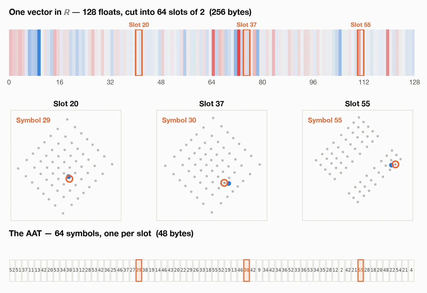
Each slot’s centroids capture the correlation two dimensions at a time. The codebooks stay small: 64 centroids per slot, not one enormous book for the whole space.

Data-science readers know this as product quantization. It drives billion-scale similarity search, and is the part of FAISS that finds near-neighbors in a corpus too big to hold in memory. A vector in $\mathbb{R}^D$ becomes k = D/2 slots. Each slot carries one symbol out of S = 2^bits — the index of its nearest centroid in that slot’s codebook. The whole code is k symbols, or k · bits bits on the wire. Write $\mathbb{A}_S$ for one slot’s alphabet, the symbols $\{0, \dots, S-1\}$. An AAT is a point in $\mathbb{A}_S^k$: $k$ slots, $S$ choices in each, the same way a real vector is a point in $\mathbb{R}^D$. The notation reads like coding theory’s $\mathbb{F}_q^n$. The subscript is the alphabet size and the superscript is how many symbols you string together.

For 64 slots of 6 bits each, the AAT is $64 \times 6 = 384$ bits, or 48 bytes: a point in $\mathbb{A}_{64}^{64}$. Compare to the vector it came from: 256 bytes in the 16-bit floats. A fifth of the size. A saved byte is never stored, never crosses a memory bus, and never draws energy.

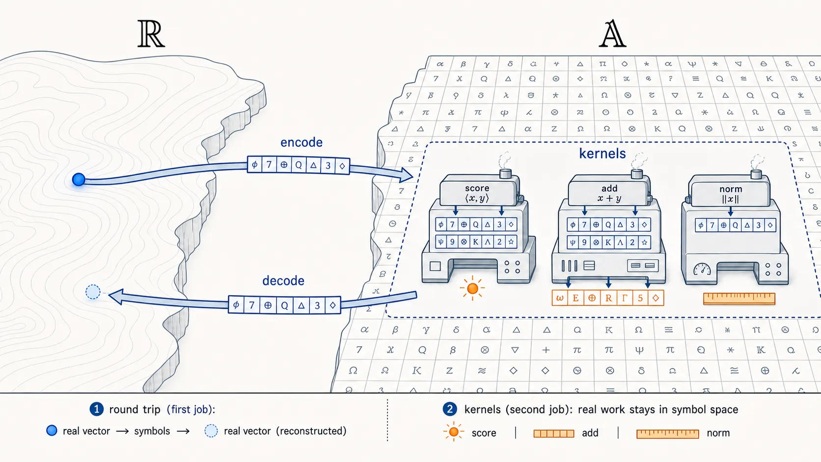
kT-RAM accepts AATs and nothing else, so all computing on this hardware happens in AAT space, $\mathbb{A}_{S}^{k}$. Models (at this time) are trained and shipped in $\mathbb{R}^D$. We had better be good at going back and forth:

$$\mathbb{R}^{128} \;\xrightarrow{\ \text{encode}\ }\; \mathbb{A}_{64}^{64} \;\xrightarrow{\ \text{decode}\ }\; \mathbb{R}^{128}$$

An encode–decode pair is a codec, the same word and much the same job as the audio and video codecs that pack a symphony into an MP3 and get it back out. We need an AAT Codec library and tool set, which is the goal of this chapter. The product-quantization codec we just assembled is our first one, Codec A.

Codecs out of $\mathbb{R}$ and into address space are all over machine learning now. The FSQ and BSQ image tokenizers round onto uniform rulers or take the sign of each axis. The neural audio codecs behind modern voice models give every few milliseconds of sound a small stack of addresses.

A codec has two jobs. The first is the round trip: encode to $\mathbb{A}$, decode back to $\mathbb{R}$, lose as little as possible. The second is kernels, mathematical operations run directly on the codes in $\mathbb{A}_{S}^{k}$, with no decode at all. Score two vectors against each other, sum them, take a norm, all in symbol space. These kernels take fewer elementary operations than the float versions they replace, touch narrower numbers, and read from tables that fit in hundreds of bytes. We convert to AATs so kT-RAM can assimilate transforms. The codes turn out to be worth computing on in their own right.

Reconstruction Loss#

Take a vector from the model, encode it, then decode it straight back to $\mathbb{R}^{128}$: look up the centroid at each slot’s address and lay them end to end. Measure how close the result is to the original.

We ran Codec A on real activations from a working transformer, Qwen3-0.6B. One middle layer, codebooks fit on one split of the data and scored on another it never saw. The measure is cosine similarity. At 1.0 the decoded vector points exactly where the original did. Lower means it drifted.

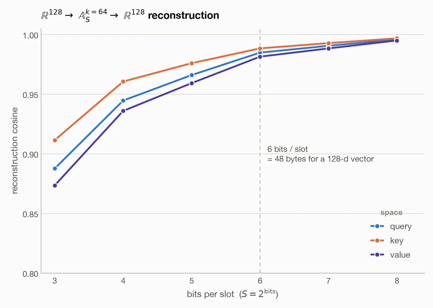
At six bits we land near 0.98 cosine. Most of the fidelity for a fraction of the size. One caveat: cosine only checks direction. A code can get the direction right and the length wrong. Parts of a transformer lean hard on length, so the next chapter watches both.

Whole images to AATs#

Codec A works on any vector, not only a transformer’s. The 28×28 Fashion garments from the last chapter are 784-number vectors, so a garment can be cut into slots and addressed like anything else. Chapter 6b already did a version of this. It cut each garment into sixteen 7×7 tiles and gave every tile the address of whichever learned feature won that tile’s read, so a whole garment came back as sixteen symbols. Slots and tiles are the same move at two scales.

Let’s try another way. Instead of breaking the image into pieces, encode it whole. Keep the shape of $\mathbb{A}_S^k$, $k$ books with $S$ entries each, and change what an entry represents. An entry is now a full 784-number image, a faint ghost of a garment rather than a piece of one. It is not a centroid. Nothing clusters around it, and on its own it is not meant to look like a garment. It is one term in a sum. Sparse coding calls it an atom. The code holds one address per book, and the decode adds the $k$ selected atoms. Making change works the same way. To reach $20.37 you go down a row of compartments and take exactly one option out of each: one twenty, no tens, no fives, one quarter, one dime, two pennies. You write down your choice at each compartment, not the amount, and adding your picks back up returns the amount. The large denominations get you most of the way there and the small ones settle the remainder, which is what the early and late books do here. The difference is that these denominations are not 25 and 10 and 1. They are fit to the garments they have to add up to. Every symbol now influences every pixel.

The books are fit, and the fit is k-means one level up. k-means assigns each point to its nearest centroid, then moves that centroid to the mean of its assigned points, and repeats. Here the assign step encodes every training garment, so each one ends up with $k$ addresses. The move step then changes every atom to whatever makes the sums it appears in come out closest. The two repeat. The full recipe. Average every training garment into one mean image and subtract that image from all of them, so the code represents each garment’s difference from the average, and the decode adds the mean back at the end. Seed each book by running k-means over those differences. Every book gets the same data, all 784 numbers of every difference, unlike a slot codec where a slot’s k-means sees only its own two columns, so at the start the books differ only in where their k-means happened to land. Then alternate two steps. The first walks the books in order and lets each one pick the atom that best cancels what the earlier books left unexplained. The second freezes those addresses and rewrites the atoms, with least squares picking new values for all of them at once to minimize the total error over every training garment. It never looks at the old atom values, because the frozen addresses already carry every choice those atoms drove. Both steps push down the same error and neither can raise it, which is why the loop settles and the books specialize apart. The one difference is that a garment is rebuilt from a sum of $k$ atoms rather than a single centroid, so the move is a joint solve instead of an average. Two atoms that keep turning up in the same garments’ codes have to divide the work between them.

The move step makes an atom look like a garment. An atom is a term in the sum of every garment whose code holds its address, so the solve drives it toward the structure those garments share. Anything else it carried would throw all of them off at once and raise the error being minimized. The early books face the whole garment and take the silhouette, and the later ones face what is left over and take the detail. The figure below uses $k = 128$ books of $S = 16$ atoms, so a garment becomes a point in $\mathbb{A}_{16}^{128}$, or 512 bits, 64 bytes.

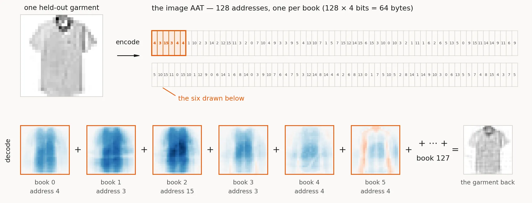
This is the additive family of codes, and it is not new. Babenko and Lempitsky named additive quantization in 2014, the two-step fit is the loop dictionary learning has always used, and the family now carries frontier LLM weight compression, recommender item addresses, and production speech codecs. What these codes cost, how far the fit can be pushed, and how they measure against the patch route is the next chapter’s focus. The gray-scale garment reconstructions at the end of Chapter 6b came out of a network using a two-level version of this additive AAT encoding.

Staying in AAT space#

Both AAT encoding constructions give us a way from $\mathbb{R}$ to $\mathbb{A}$ and back. Return now to the transformer, where the round trip is only the start of the problem. Every encode and every decode costs time and energy, so once we encode we stay in AAT space as long as we can. We decode when an operation or the end result needs real numbers.

kT-RAM consumes and produces AATs. To assimilate a transformer (as one example) we need a plan for the operations that sit outside the layers a neural lane can represent:

• inner products between vectors — the attention score
• vector length — the norm, used in normalization and scoring
• weighted sums of vectors — the attention output, blending many value vectors into one
• addition — the residual stream running up the spine of the network

None of these operations use the learned parameters, but a transformer cannot work without them. The projections that make the queries, keys, and values are big matrix multiplies, and so is the MLP between attention blocks. Those learned parameters are what the kT-RAM neural lanes can assimilate. These four other operations run between the lanes, and the longer the context, the larger their share of the arithmetic.

That leaves two routes. Decode back to $\mathbb{R}$ and re-encode later, or run these operations directly in AAT space. The second options sounds great, but how do we do that?

Take the attention score. It is the inner product of a query vector and a key vector: multiply the two element by element and sum the products. The obvious route decodes both vectors back to $\mathbb{R}^{128}$ and performs 128 multiply-accumulates. An AAT codec kernel can do the same job with no multiplies at all. Precompute the inner product of every centroid pair, slot by slot, and store them in lookup tables. Scoring two codes is then 64 table reads and 63 additions. Vectors are never decoded. This is standard practice, not something we invented. Jégou, Douze, and Schmid’s 2011 paper Product Quantization for Nearest Neighbor Search, linked above, calls scoring two codes through a centroid-to-centroid table symmetric distance computation. The asymmetric variant, where one side stays in $\mathbb{R}$ and only the stored side is coded, is what FAISS and Google’s ScaNN run in production billion-scale search. In gates and energy, a multiply-accumulate is one of the more expensive things digital hardware does, and a table read and an add are among the cheapest. A commodity processor complicates that ranking. Its multipliers are the most optimized machinery on the die, and a table read is a memory access. Chapter 7c comes back to which hardware collects which number.

Not shippable…yet#

Codec A’s cost shows up in two places. First, the lookup tables are not small. Scoring queries against keys needs a table of $S \times S$ inner products for every slot: $64 \times 64 \times 64$, over a quarter-million entries for one layer’s score kernel. Second, encoding is worse. Finding each slot’s nearest centroid means measuring the distance to all 64 of them, so encoding one vector costs thousands of multiplies. Getting into $\mathbb{A}$ takes far more arithmetic than the 128 multiplies the kernel saved!

Codec A works but it is unshippable. Can an AAT codec keep this fidelity with tables small enough to sit next to the hardware and an encoder cheap enough to run on every vector coming down the residual stream? That is the next chapter.