Chapter 6b: The Unsupervised Basis Encoder

In Chapter 6 we reviewed the kT-RAM supervised classifier routine: read every lane, drive the labeled lane’s weights high, drive the confident-wrong weights low, and hand the rest to the regularizing ‘FF-RZ’ instruction, giving the equivalent of established machine learning methods like logistic regression.

Take the label away and the routine still runs, with one substitution. Show the lanes an example AAT pattern, they read back a voltage per lane, the loudest wins, and that winner becomes the target: reward the winning lane, depress the confident losers, repeat.

Run that over unlabeled AATs and each lane drifts toward a prototype, a little pattern it comes to represent, so the lanes turn into a codebook: a small dictionary of patterns whose “code” for any input is the winning lane’s index. The idea is old, well understood, and goes by several names — competitive learning, online vector quantization, learning a dictionary. A plain winner-take-all competition collapses, though, unless we constrain how much a winner takes.

pip install "git+https://github.com/knowm/ktram-neural-core.git#subdirectory=python"

The code is in examples/basis-encoder.

Rich get richer#

Picture the first few example AATs. Some neural lane, by luck of its starting state, reads a hair louder than the rest and wins at random, so we reward it, which makes it read louder still on anything similar and biases it to win the next round, and the next. An early accident of circumstance compounds into a monopoly, and a lane that never wins is never rewarded. Run it long enough and a bank of sixty-four lanes collapses to two or three, even one answering for everything, and the diverse codebook you wanted, a collection of unique prototypes, degenerates into a monopoly saying one thing. I call that the null state, reached in short order by pure rich-get-richer competition.

We need to reward winners without collapsing the system. Rewarding a winner lets that lane establish its prototype and settle on what it represents, while competition between lanes, each holding its own ‘synaptic territory’, produces the decision boundaries that maximize the support vectors between patterns. Winners must win, and exclusion caps the positive feedback spiral ending in the null state.

Exclusion (of the rich)#

Exclusion applies to the winner: a lane that already won once during a defined cycle period steps aside and takes no second reward until the others have their turn, and without it a single lane wins everything and locks the rest out of the codebook for good. A “cycle” is a defined period, measured in input patterns seen, plus one addition discussed below.

That one rule keeps the rich in check and lets a codebook form. The early leader still wins its first example, then steps aside, and the next reward goes instead to whoever reads highest among the lanes that haven’t won yet, which spreads the learning across the whole bank. In hardware the mechanism is one bit per lane: won this cycle, or not.

Write $\mathcal{L}$ for the lanes in the group, $y_\ell$ for the sub-threshold read of lane $\ell$, and $W \subseteq \mathcal{L}$ for the set of lanes that have already won this cycle; the read winner is $w = \arg\max_{\ell \in \mathcal{L}} y_\ell$, and exclusion gates the reward on membership in $W$: feedback is issued when $w \notin W$, and withheld when $w \in W$.

Recruitment (of the poor)#

Exclusion keeps the rich in check, but it doesn’t guarantee that a lane starting in a bad spot ever gets going: such a lane can lose every read forever, sit at its initial state, and contribute nothing. The same random initialization that handed the rich their privileged start can work the other way and keep a lane from ever winning, so a second rule pushes from the other side.

When a long stretch of updates goes by without the cycle completing, we stop waiting and force it, rewarding the highest-reading lane among those yet to win even though it did not win this round. Gather winners for a while, rewarding each once, and once a defined cycle time passes, abandon the wait and start recruiting the lanes yet to win anything. That pulls idle lanes into service, every lane gets used, a diverse basis set forms, and in hardware this is a counter.

Recruitment reads the same set $W$ the other way. Let $n$ count the updates since the cycle last cleared and $G$ the gather_abandon threshold: once $n \ge G$ with lanes still idle, the group stops waiting and rewards the highest reader among the lanes yet to win, so lane $r$ joins $W$ with an FF+RH reward whether or not it won the read.

The cycle#

Both rules run on the same bookkeeping. Each lane carries one bit recording whether it won this cycle, and once every lane has won, the cycle completes, the bits clear, and competition restarts. Exclusion checks that bit before issuing a reward, and the number of bits set tells us whether the round stalled. A counter and a threshold we call gather_abandon set the cycle time, the point where we abandon gathering winners: when the round’s counter hits that threshold we start force recruitment, and once all lanes have won, the cycle restarts.

The routine#

We start with a low-voltage read, FFLV, over all lanes, return the lane with largest $y$ as output, and gate the reward by the two mechanisms above.

def adapt(x):                        # one unsupervised update on input AAT x
    y = [read(x, lane, FFLV) for lane in group]   # 1. decide — sub-threshold, disturbs nothing
    winner = argmax(y)

    if not won_this_cycle(winner):   # 2. exclusion
        correct(x, winner, RH)       #      reward the winner       — FF then RH (up)
        for lane in group:           #      depress the fired losers — FF then RL (down)
            if lane != winner and y[lane] > 0:
                correct(x, lane, RL)

    if cycle_stalled():              # 3. counter>gather_abandon, start recruitment
        r = highest_reading_unwon_lane(y)
        correct(x, r, RH)            #      pull an idle lane in     — FF then RH (up)

    mark(winner); tick_cycle()       # 4. one bit per lane; clear the cycle when all have won

def correct(x, lane, reverse):       # the ONLY place a forward instruction is issued
    evaluate(x, FF, lane)            #   forward read at full voltage — this one adapts
    evaluate(x, reverse, lane)       #   its paired reverse — no path ever leaves an FF unpaired

The FFLV instruction is the sub-threshold read, FF is the same read at full voltage and will decay the conductances slightly, and RH and RL are the reverse instructions for driving a lane high and low, respectively (review the kT-RAM instruction set in Chapter 4b). Every forward instruction pairs with a reverse, so a correction is FF+RH (the winner) or FF+RL (the confident runner-ups), the same instruction set as the supervised classifier’s FF → RH/RL/RF minus the true-negative RF case. This basis encoder touches only the lanes that spoke up and leaves the rest of the bank alone. kT-RAM allows many routines; this one works and we can measure it, but it is not the definitive basis encoder, and others trade differently between codebook quality, instruction count, and hardware bookkeeping. On sixty-four lanes, most get no instruction on a given update.

Forming & Sharpening#

Run the cycle above and every lane stays in play, pulled toward a prototype, but recruitment keeps propping up lanes the data doesn’t support. Asking 64 lanes to learn a basis set when only 32 patterns exist makes the codebook ‘smear’: a couple of lanes answer for two things at once, and the cost shows up in purity, growing with the mismatch. Holding recruitment on throughout, 64 lanes score 0.88 on a source of 48 patterns, 0.84 on 32, and 0.75 on 16.

To resolve the smearing we run training in two phases.

We form first, using the cycle routine above, with recruitment on so the bank populates, a full and varied set of prototypes develops, and nothing gets starved before it has a chance to specialize. Partway through we turn recruitment off and let the lanes ‘sharpen’, so nothing props up a lane that quit winning: at a cycle’s end (counter>gather_abandon) we reset rather than force recruitment. The lanes that keep winning grow crisper, the ones recruitment alone kept alive stop being rewarded and fade out, and the codebook prunes down to what the data supports.

One bank runs below on binarized Fashion MNIST images, with sixteen lanes and no labels, forming and then sharpening right at the end.

Does it work?#

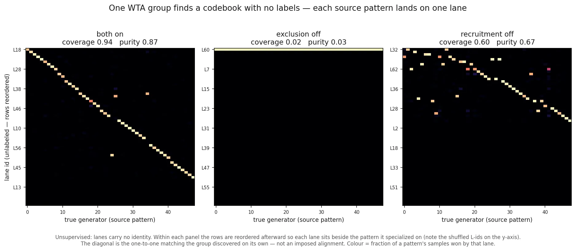
On a synthetic source we know the true prototypes that generated the data, so “clean” is a measurable quantity: what fraction of the true prototypes got claimed by a lane, which we call coverage, and how single-minded each lane stayed, its purity.

Both numbers come from one tally table. Freeze the group, run it over a batch of samples whose true source pattern we know, and each time a lane wins a sample add one to the cell for that lane and pattern. The result has one row per lane and one column per true pattern, where cell $M_{\ell g}$ counts the times lane $\ell$ won a sample from pattern $g$. A perfect codebook has one bright cell per row, each in a different column, the diagonal in the figure below.

Purity is the fraction of a lane’s wins from its single most common pattern, averaged over the lanes that won anything, and coverage is the fraction of true patterns that at least one lane claims as its most common win.

If two lanes claim the same pattern it counts once, and a pattern no lane claims is missing from the codebook, so a group that merges several patterns onto one lane, or leaves patterns unclaimed, reads as low coverage, while a lane answering for two at once reads as low purity. Utilization is the fraction of lanes winning anything.

With both exclusion and recruitment on, coverage and purity run high. Knock exclusion out and one winner remains, the degenerate null state; knock recruitment out and fewer than half the lanes ever win a read, so coverage drops from 0.94 to 0.60. Every pattern still finds a winner, so one-to-one recovery is what breaks: thirty survivors cap coverage at thirty of forty-eight patterns. Exclusion protects purity and recruitment protects coverage, and since recruitment gains coverage at a small cost in purity we keep it on to fill the bank and give every lane a chance, then take it off to refine and sharpen.

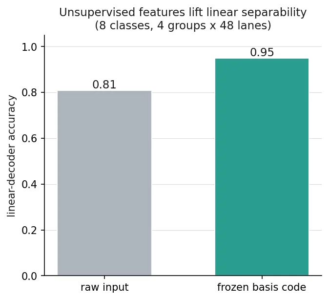
On the synthetic source the code is also markedly more separable than the raw input: a single linear read climbs from about 0.81 on the raw signal to 0.95 on the frozen basis code, which is what a good learned representation buys you.

Patch Codebook#

The same routine learns a codebook over Fashion MNIST sub-patches instead of whole images, shown below.

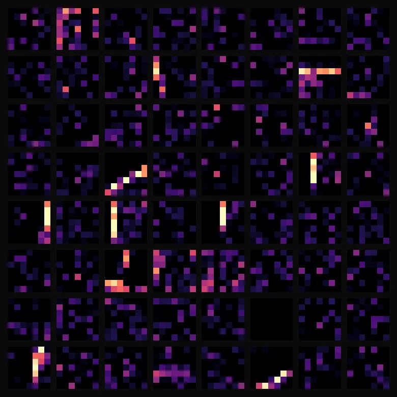
Each tile is one lane’s prototype pattern, the same things sparse-coding folks have extracted from natural images for thirty years: oriented edges, bars, corners, little scraps of texture.

One group covers one 7×7 tile, so a 28×28 image takes sixteen of them, each with its own sixty-four lanes and codebook, and reading all sixteen and keeping each winner returns the image as sixteen integers, the tuple that is the image’s AAT.

Sixteen integers now stand in for 784 pixels, and the squeezed code still carries enough for a lane to read the garment’s class off it and a bank of lanes to rebuild the picture. Both are the routine we already have, pointed at a different target, and the second closes the loop into a generator.

A simple kT-RAM auto-encoder-decoder-classifier network#

Everything until now has been one group of lanes at a time. We now build and train our first “multi-module” kT-RAM network from three parts, two of which you have met: the supervised classifier from Chapter 6 and the basis group from the top of this chapter. The new part is the wiring.

Topology#

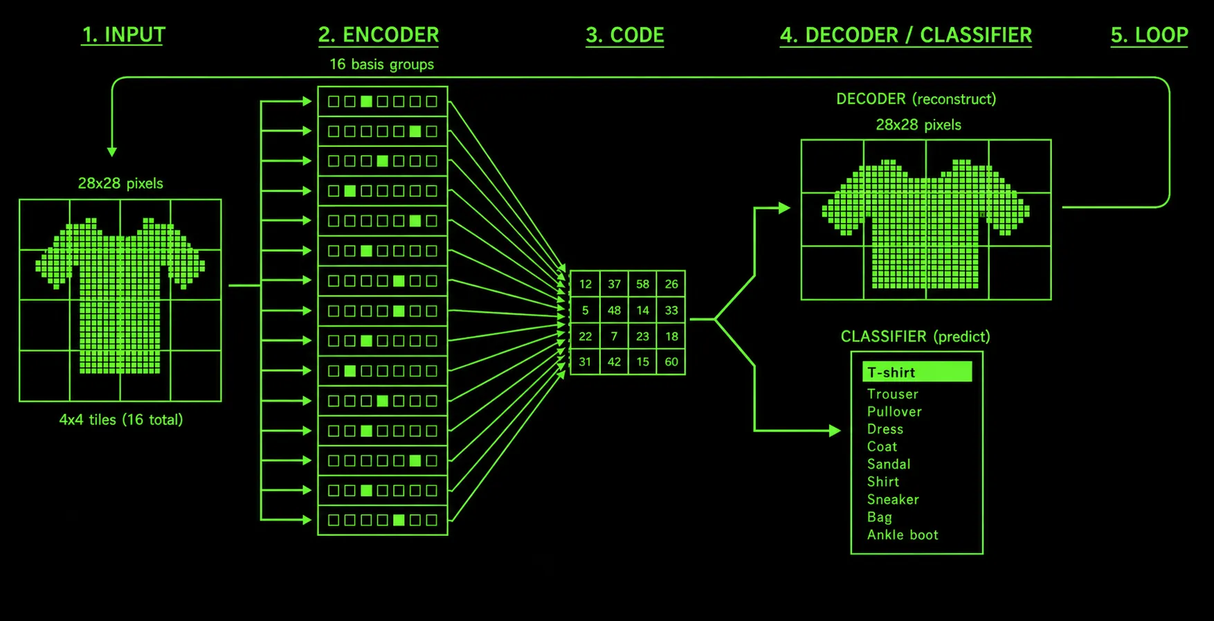
Start with a Fashion MNIST image of 28×28 pixels and threshold it at its own mean gray level, so each pixel is either white (1) or black (0) and the whole picture is 784 bits, then cut it into a 4×4 grid of sixteen non-overlapping 7×7 tiles. Tile 0 is the top-left corner, tile 3 the top-right, and tile 15 the bottom-right.

The encoder is sixteen basis groups, one per tile, each a 64-lane WTA group of the kind from earlier, and group $g$ sees only tile $g$, never anything else. Its input AAT has 49 spaces, one per pixel, each with two addresses, white or black, so sixteen groups give sixteen integers and that 16-tuple is the image’s code, itself an AAT of sixteen spaces with 64 addresses each. 784 bits go in and sixteen integers come out.

The decoder takes the encoded 16-integer AAT and outputs predicted pixel values from one kT-RAM core of 1,568 lanes, two per pixel, one for white (1) and one for black (0). Every decoder lane reads the full sixteen-space AAT, so it holds $16 \times 64 = 1{,}024$ synapses, and two such lanes form a WTA group predicting the pixel value, 0 or 1. Because both of a pixel’s lanes read every tile’s code at once, a change in one tile’s winner can propagate across the picture.

The label read-out is ten lanes, one per Fashion class, reading the same sixteen-space AAT at 1,024 pairs per lane, and like the decoder it is an instance of the Chapter 6 classifier.

This network holds 1.7M differential pair synapses, and the decoder owns nearly all of them: the encoder is ~100k synapses and the read-out ~10k.

Training#

The encoder trains first unsupervised, each group running the adapt loop above over 12,000 training images with gather_abandon = 96, and is then frozen.

We then run the frozen encoder over 8,000 training images once and keep the 8,000 AAT codes, on which the decoder and label read-out both train for four passes. The decoder’s target for pixel $p$ is the true bit of pixel $p$ in the training image, and the read-out’s target is the class label.

Inference#

Once frozen, the entire network operates on FFLV reads: an image becomes a sixteen-integer AAT, and that AAT becomes 1,568 decoder reads and 784 bits, plus ten read-out reads and a label.

Closing the loop#

The decoder’s output is a 784-bit image, exactly what the encoder takes as input, so we feed it back to itself: the machine’s state is an image, and one step is encode then decode. With no read noise every read is a deterministic map from images to images, and the picture falls into an image that encodes and decodes back to itself within a few steps.

The temperature is the read-noise gain on the encoder’s FFLV read. Each of the 1,024 encoder lanes draws its own noise on every read, at the width $\sigma(V)$ from the read-noise chapter, and the group’s winner is whichever lane reads highest after that noise, while the decoder and read-out stay sharp, so encoder noise is the one knob the widget exposes.

Turning up the temperature#

Start with an image, encode it, decode the code back to an image, encode that, around again. At low noise the loop quickly settles onto an image that encodes and decodes back to itself, a fixed point attractor: a clean garment the encoder and decoder agree on, which the loop falls into from almost any start.

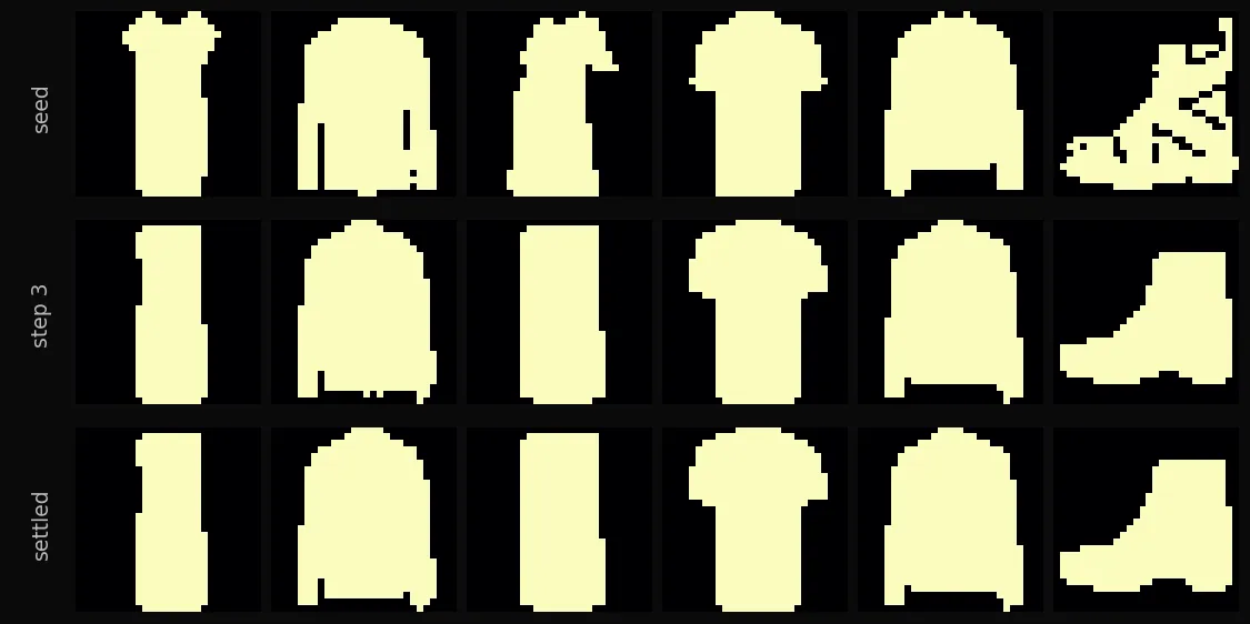
Every kT-RAM read carries the kT-bit’s own read noise, the thermal noise on the sense line, and the read voltage is our dial for it: turn the voltage down and the same read gets louder with noise. The winner is then sampled, weighted toward the loud lanes but free to grab a near-runner-up when noise tips it over, and that noise width $\sigma(V)$ is our temperature, the thermal-plus-flicker noise introduced from Chapter 3b. At zero noise the loop settles and holds a garment attractor; turn it up and the winner starts to wander, the code drifts, and the decoded image morphs, a boot morphing into a sneaker and a coat into a dress. Turn it back down and it snaps into the nearest clean attractor.

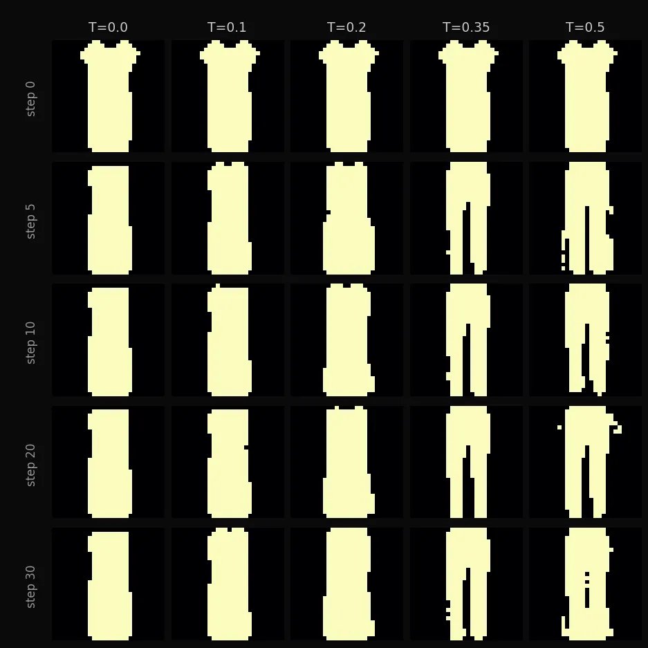
Run the loop yourself in the widget below.

Drag the temperature up to watch it explore, drop it to watch it settle. Click any patch to open its codebook and see the sixty-four features it was choosing between, the current winner boxed, and click ‘Codebook’ to return to the generated image. The header names the class.

What this maps to#

This series maps machine learning methods onto kT-RAM neural lanes, and we are typically not reinventing these algorithms or techniques so much as learning what the hardware is capable of, one capability at a time.

The winner-take-all update is called competitive learning and the codebook of prototypes is a vector quantizer. Exclusion is a hard, cycle-scoped version of DeSieno’s conscience, the 1988 trick of penalizing a unit that wins too often so the rest get a turn, and recruitment is the online form of the dead-unit reinitialization k-means does on an empty cluster. The learned patch features are the sparse-coding dictionary without the L1 penalty or gradient descent, and the encoder-and-decoder loop, code in and image out, is an auto-encoder, one of the oldest unsupervised architectures there is.

The basis encoder takes its place next to the classifier as a second L1 module, a named, reusable routine executed over kT-RAM neural lanes, and the set now holds memory, logic, a supervised classifier, and an auto-encoder.

Sneak peek#

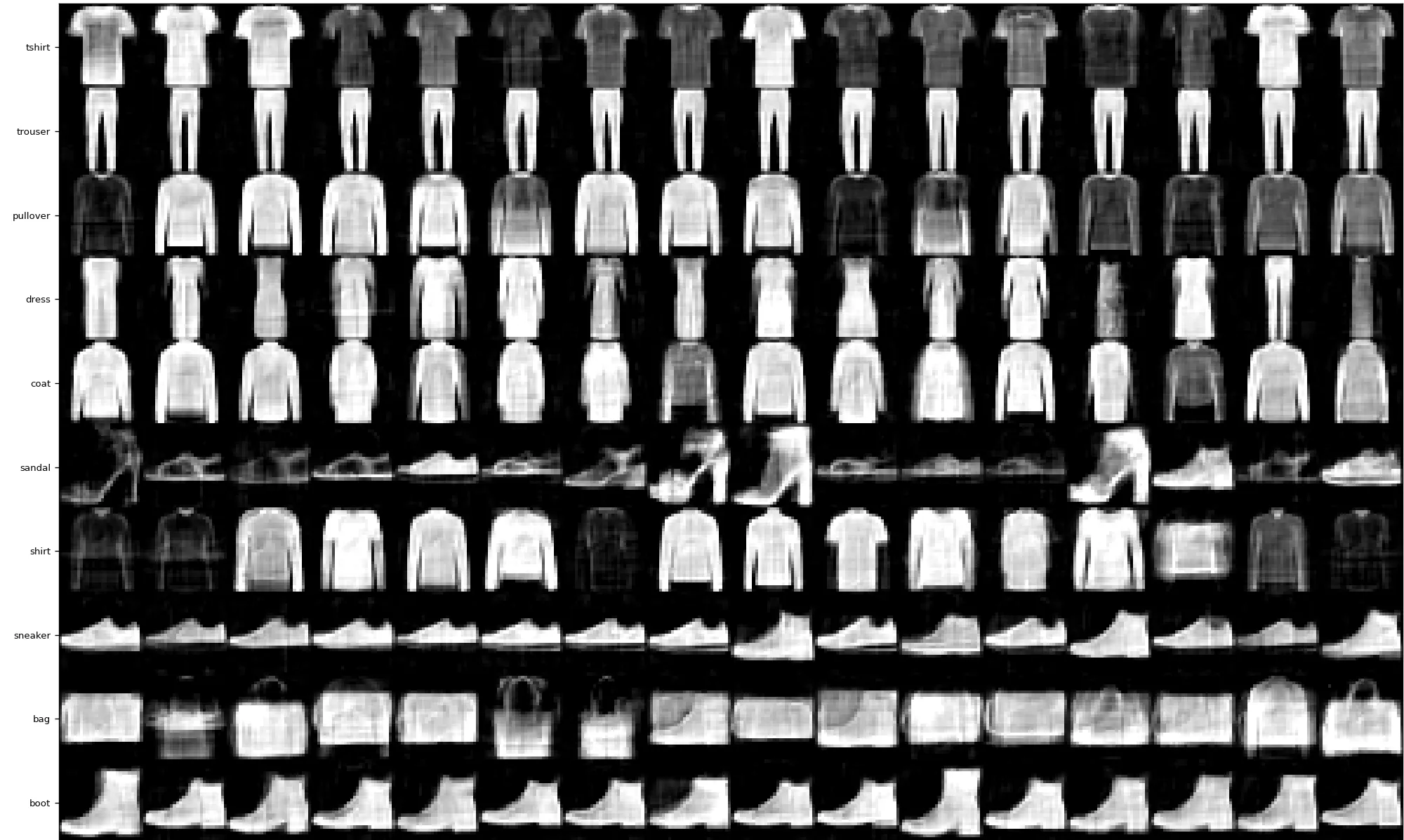
This chapter’s generator is deliberately small: binary pixels, sixteen integers, one encoder, one decoder, and one classifier. I could not leave it there, so I spent a weekend on larger full-bit-precision kT-RAM image generation networks, and the images below are samples from one. I’ll write it up in a future chapter, once we lay down chapters on more sophisticated AAT encoding, and it is a tangent to my stated goal of neural network assimilation, so I can’t get too distracted!

Next: Chapter 7: The AAT Codec