Chapter 4b: The Neural Lane Emulator

At the end of Chapter 4 I said the next thing was code — so let’s begin. I am an old Java-native, and the old “Knowm API” is all Java. I’ve used AI to help translate the work into Python and notebooks. The point is teaching and intuition, not speed: a small, readable emulator we can run experiments on and reason about. As this series progresses we will run bench tests, tweak the emulator as needed, and try to keep our actual built hardware synced up with the code.

One install line, and one notebook you can open in Colab and start poking at.

pip install "git+https://github.com/knowm/ktram-neural-core.git@chapter-4b#subdirectory=python"

The emulator#

The package mirrors the neural core we are going to build, so the object model reads like the hardware from the outside in:

• Core — the kT-RAM implementation as specified by the neural lane concept: the unit-crossbar geometry, the device model, the initial conductances, the control voltages. You address it the way you address the hardware, with AATs. A core holds one or more neural lanes.
• NeuralLane — an array of UnitCrossbarPairs. Each pair handles one entry of the AAT tuple, and all of them are coupled together and read through one 2-1 divider network.
• UnitCrossbarPair — one differential pair of unit crossbars, an a-side and a b-side. When selected, it exposes a single signed synapse to the lane.
• UnitCrossbar — the crossbar array that couples one selectable device at a time.

You address the lane the way the hardware does. A kT-bit selection is an AAT — a tuple, one entry per pair. Chapter 4 covered why: the tuple is the wiring, so the encoding and the physical layout are the same object, pin for pin.

Two knobs change what a core is made of. The first is the device model, i.e. a model of the memristors. Swap it with one word: float is an idealized device, byte an 8-bit counter-like model, and mss and rs are more accurate stochastic models of memristors. The second is the crossbar fidelity — how much of a real array’s mess you simulate. ideal reads each device as if it sat alone; physical (coming later) adds the current leakage and wire resistance a real crossbar actually suffers. We will likely be taking more careful measurements of real devices and updating our memristor models as we progress. For now the parameters in the code are simple whatever happen to be in my old Java Knowm API, which got copied over.

Nothing about the device is hardcoded into the lane. A device model carries its own physics constants; the Core owns the operating voltages and the pulse width and hands them to the device when it drives it. The MSS model in particular carries a full settable profile, so it can be fit to the measured physics of a real device. Contrary to what is expected, the MSS model is not a model of Knowm SDC devices. I came up with the MSS concept and model years prior. Their are some real shortcomings with it (and many other memristor models).

This is the first release, so the scope is deliberately small. You get the single-lane core, the four device models, the shared 2-1 readout, the full instruction set, AAT selection, and pulse-width drive.

A single synapse#

Set the spaces-per-lane and the lane count to one and the lane collapses to a single differential pair: one device on each side, selected by the fixed AAT z = (0,). That is the entire API surface for now.

from ktram_neural_core import Core

core = Core(1, 1, spaces_per_lane=1, num_lanes=1,
            model="float", init="medium", seed=1)
lane = core.lane(0)
z = (0,)                        # the AAT: address 0, the one space

y      = lane.evaluate(z, "FF") # forward read -> the weight, in [-1, 1]
ga, gb = core.read_gab(0, z)    # peek at the two conductances (debug/emulator only)

evaluate(z, instruction) runs one instruction per call. That is the whole loop — and the instructions are the vocabulary.

The instruction set#

Fourteen instructions make up the set, and every one is a two-letter code. The first letter is the drive direction: forward (F) or reverse (R), the polarity of the voltage across the pair. The second letter is the operation, and it is either a read or a feedback.

A read floats the y node and measures the synapse’s signed output — that floating is the second F, for float. There are four: forward and reverse, each at full voltage or held below the switching threshold (LV). The full-voltage reads drive the devices as they measure, so they adapt the pair a little every time; the sub-threshold reads report the weight without moving it.

A feedback clamps y to a fixed voltage instead of floating it, and that voltage nudges the two conductances. The second letter picks the direction. H and L are supervised — you choose which way the weight moves, H up toward +1 and L down toward −1. U and A are unsupervised — they take their direction from the last read, which is held until the next read recomputes it. U reinforces the current sign (Hebbian); A opposes it (anti-Hebbian). Z applies nothing.

The forward and reverse codes for an operation move the weight the same way but treat the magnitude oppositely. Forward feedback accumulates — it adds conductance, so the magnitude grows and the pair counts evidence. Reverse feedback depletes — it lowers the opposite conductance, a leaky average that shrinks the magnitude.

The forward/reverse split runs deeper than Hebbian versus anti-Hebbian. A memristor moves up in conductance under one polarity and down under the other, between a hard floor and a hard ceiling. Drive a synapse with forward instructions alone and both devices climb until they saturate against the ceiling; drive it with reverse alone and they bottom out on the floor. Either way you have lost the synapse — both devices pinned at a rail, no range left to represent anything. That is why every working cycle typically pairs a forward operation with a reverse one, each push toward a rail answered by a push back, and that constaint ‘flip-flopping’ is what holds the pair in its usable middle.

Inertia and evidence, on one synapse#

Chapter 3b read two properties off the magnitude: it is the weight’s inertia, and it is a count of evidence. Here is how you get both back out of the emulator, on a single synapse.

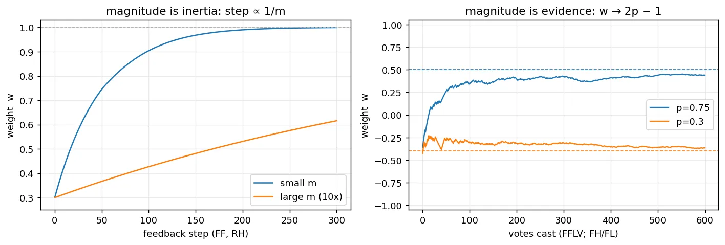
Left is the inertia: same starting weight, ten times the magnitude, a tenth of the step — the magnitude sets the effective learning rate, which falls as 1/m — so the light pair races to the rail while the heavy one crawls. Right is the evidence count: vote a stream of yes/no into the pair and the weight settles on the running frequency, 2p − 1. Nobody wrote the annealing schedule and nobody stored the vote count — both just fall out of the weight magnitude for free. Chapter 3b has the why; this is how you reproduce it in code.

The read is a sample#

Every read above came back as a clean number — the exact ratio of two conductances. A real kT-bit cannot hand you that. Each device sits at a temperature, and a conductor at temperature T hisses. That hiss rides on the read, and the emulator models it. Read noise is on by default, at room temperature: a read returns the weight with a little scatter on top.

The scatter is referred to the read value y. That y is the lane’s output — the one number the 2-1 divider returns when you read one or more synapses together — and for the single pair here it is just the weight w. It sums two mechanisms in quadrature Adding by the Pythagorean rule: the combined size is √(a² + b²), not a + b. It is the right way to add two independent noise sources, because their fluctuations are uncorrelated and partly cancel rather than stacking head to tail. :

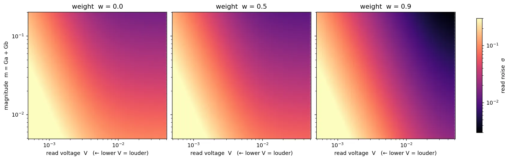
• Thermal (Johnson–Nyquist) — additive noise on the signal. It grows as 1/|V|, so lowering the read voltage shrinks the signal while the hiss stays put and the read gets louder; it also scales with √T and falls as 1/√m. A small floor.
• Flicker / RTN — the multiplicative conductance flutter (1/f noise) that dominates the read on real memristors. Flat in read voltage — a floor the voltage dial cannot drop below — falling as 1/√m, and carrying a factor (1 − y²): loudest when the pair is undecided at y = 0, silent at the rails where a confident pair reads clean.

The floor is flicker — the weight and the magnitude set how high it sits, and no read voltage gets you under it. Thermal is the dial above it. In principle you turn it two ways — with temperature, since it scales as √T, or with the read voltage — but you rarely heat a computing device on purpose, so the read voltage is the knob we use. Leave the voltage at full and thermal stays well below the floor, so the read sits at the floor; turn it down and thermal climbs until it clears the floor, and from there the read only gets louder. Hold the weight fixed, sweep the read voltage against the magnitude, and we can construct a nice heatmap:

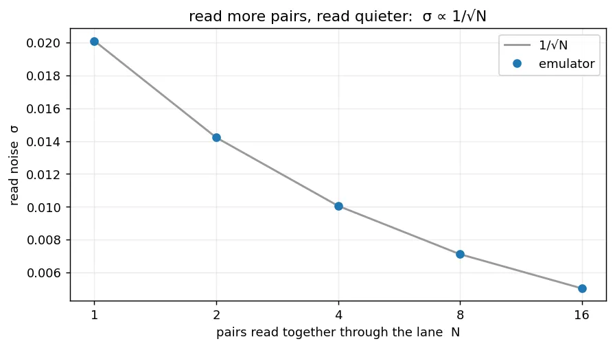
That map is for one pair. Read several equally-confident pairs through the same divider and their noise pools — the read falls as 1/√N, the wire doing inverse-variance weighting for nothing.

A sub-threshold read is the one you sample with — it will not erode the weight it is reading. The kT-bit is a random source you can write a bias into. Park the pair at the balance point and the clean read is zero, so the sign of a noisy read is a fair coin pulled straight from the device’s own noise. Write a weight first and the coin tilts: the probability of a positive read is the Gaussian CDF of the weight measured in units of the read noise, P(+) = Φ(w/σ).

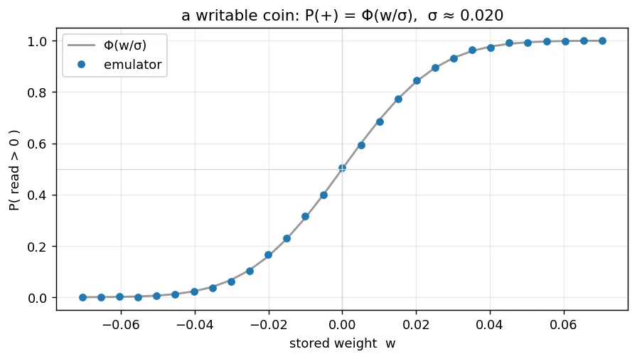
The stored weight is the bias, adaptive and written by the feedback instructions and re-writable on the fly. The noisy read is the draw — generative, a random bit whose probability you programmed. A sub-threshold read to sample, a feedback to adapt, and the device threshold keeps the two from colliding. NThe randomness is the device’s own hiss, and the bias is a number you wrote or that was learned.

What we covered#

Everything here ran on one differential pair. The package mirrors the hardware — Core, NeuralLane, UnitCrossbarPair, four device models — and a single lane collapses to one synapse you drive with fourteen two-letter instructions: four reads and ten feedbacks.

On that one synapse we watched the Chapter 3b physics come back out: the magnitude as the weight’s inertia and as a running count of evidence, the read as a noisy sample (thermal over a flicker floor, quieter with magnitude, pooled across pairs as 1/√N), and the writable thermal coin P(+) = Φ(w/σ). Two conductances and a handful of codes — and selecting more pairs into the same lane is where memory, logic, classifiers, autoencoders, and random sources come from.

Next: Chapter 5: AHaH Attractors