Chapter 5: Thermodynamic Logic Gates

In Chapter 3b we found how much falls out of just two memristors wired against each other — a kT-bit. Their balance is a weight; their total is a magnitude which is at once the weight’s inertia or annealing rate and also the accumulated evidence behind it, and reading the pair at low voltage draws a thermal sample. Chapter 4b ran exactly one of them as a one-synapse lane and got all of that physics back out of the emulator. That a lot for single kT-bit!

So what happens when you put two kT-bits on the same lane and drive them with kT-RAM instructions? In this chapter we will focus on unsupervised AHaH plasticity, i.e. the FF-RU instruction set pair.

pip install "git+https://github.com/knowm/ktram-neural-core.git#subdirectory=python"

Two kT-bit synapses#

A two-synapse node is a lane with two address spaces — one kT-bit per space. The AAT now has two slots, and it decides which synapses are coupled to the readout on a given evaluation:

P0  = (0, None)   # synapse 0 alone        "[0]"
P1  = (None, 0)   # synapse 1 alone        "[1]"
P01 = (0, 0)      # both synapses coupled   "[0,1]"

(0, None) couples only synapse 0; the None is the enable bit set to ‘off’, an open circuit on that space. (None, 0) couples only synapse 1. (0, 0) couples both, and the neural lane output returns their activity-weighted average.

The drive is two instructions per step, and the two halves are where the name AHaH comes from — anti-Hebbian and Hebbian. First a forward read, FF, which floats the output and reports the node’s state while pulling it weakly toward zero (the anti-Hebbian half). Then reverse unsupervised feedback, RU, which takes its direction from that read and pushes the weight further the way it was already leaning (the Hebbian half). Read, then reinforce. Nobody supplies a label (thats coming in Chapter 6); the node’s own output is the teacher in the loop.

Orthogonal Inputs#

We will start with the easy case: drive the node with P0 and P1 only, one or the other at random, never both. Each synapse gets read and reinforced entirely on its own, so the two never interact. A synapse that started a hair positive reads positive, gets pushed more positive, and runs to a rail; one that started a hair negative runs to the other. Two synapses, two signs each, and $2^2 = 4$ stable outcomes. Easy.

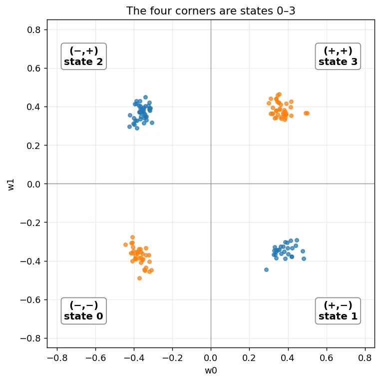
Initialize a few hundred nodes near the origin, run the cycle, and plot where each synapse pair ends up — synapse 0’s weight on one axis, synapse 1’s on the other.

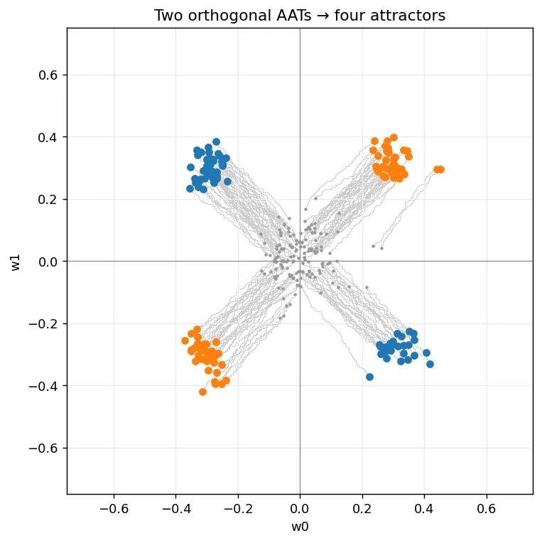
Four attractor basins, and which one a node lands in was set by the luck of its initial conductances. This is the whole of unsupervised AHaH learning in its simplest form: a weakly-broken symmetry, reinforced until it commits.

Non Orthogonal Inputs#

Those four attractors came easy because the two synapses never met. P0 and P1 are orthogonal — each one reads and reinforces its own synapse. Let the third AAT in, P01, which couples both synapses to the readout at once, and drive the node with all three patterns at random. Now a single feedback instruction lands on both synapses together, so they stop being independent.

Once they interact, naming the state by its quadrant in weight space stops being useful. We will describe the node by its decision boundary instead — the divide where its answer flips from positive to negative. A little algebra gives it to us directly. The output is $y = x_0 w_0 + x_1 w_1$, and the boundary is wherever that crosses zero:

That is the equation of a line whose slope is the ratio of the two weights, which is exactly why we call it a linear neuron. There is no constant term, so the line runs through the origin. (Two synapses make a line in a plane, three make a plane in space, and more make a hyperplane) Plot the input patterns on the same axes as that line and you can read off at a glance how the node answers each one.

There are three patterns to plot — [1,0], [0,1], and [1,1] — because there is no pattern for nothing: an input that never arrives carries nothing to learn from. Each distinct way the line can slice those three is a state the node can fall into, and they all fit on a single plane.

Each line is a state paired with its anti-state, the same boundary read in the opposite direction. Starting from random weights and driven with no teacher, which of these states does a node actually land in? Run a few hundred and count.

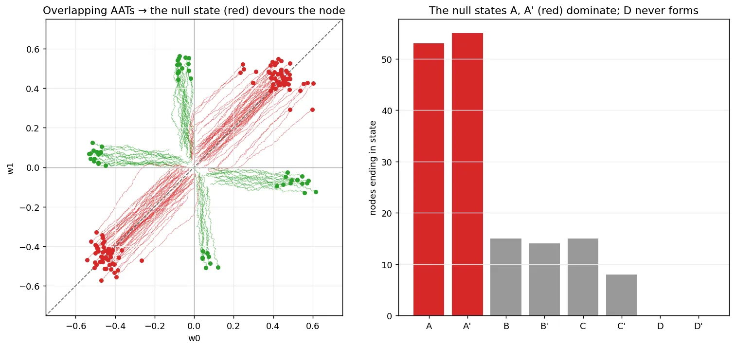
Most of the nodes slide onto the diagonal in weight space where the two synapses agree, both positive or both negative. That is state A together with its anti-state A’, and we call it the null state: it answers every pattern the same way, and it is greedy, taking roughly two-thirds of the nodes. A few escape to B and C at the edges. The bar chart also leaves room for a fourth state, D, and it stays empty — D would mean answering [1,1] differently from both [1,0] and [0,1], which takes a boundary that misses the origin, and a bias-free node has no such boundary, so it never appears.

This is what unsupervised Hebbian reinforcement does when inputs share a synapse and you are not careful. Its a version of “the rich get richer” playing out in our two kT-bit node. The pair’s joint output gets read and fed back as a unit, both synapses are pushed the same way, and the easiest agreement to reach — every pattern answered the same — swallows everything else.

Obtaining the D state#

The bar chart left one slot empty, and it is worth asking why. Here are all four states drawn together this time, with D included.

A, B, and C are the boundaries the bias-free node reached, all of them through the origin. D is the red line, and it does not go through the origin. Our node can only ever draw a line through the origin, because its output is $y = x_0 w_0 + x_1 w_1$ with no constant term. To reach it, the line has to shift away from the origin, and that takes a constant. This is called a bias: an extra synapse that fires on every pattern. Chapter 6 shows how to get one from a ConstantEncoder. An always-on input adds the same amount to $y$ every time, and that constant is exactly the offset that lets the decision line cross zero somewhere other than the origin.

Split Feedback#

Drive it with the same RU as the inputs and it becomes one more vote for whatever the node already says — another synapse agreeing with the majority — and it digs the null state deeper. It would be nice if the bias pulled the other way, so we split the feedback.

Read the whole node once with FF, the bias included. Then feed back RU on the input synapses as before, and RA on the bias — the same reverse feedback as RU with its sign flipped, anti-Hebbian instead of Hebbian, so the bias is pushed against the node’s output instead of with it. Read once, Hebbian feedback on the inputs, anti-Hebbian on the bias.

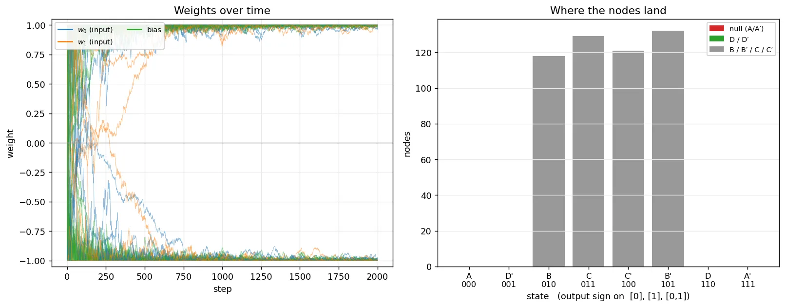
It works, up to a point: the null state is gone. A and A’, the all-one-answer states that had swallowed two-thirds of the nodes, are empty. But look at the histogram — D and D’ are empty too. A single bias started at low magnitude is enough to break the null collapse, and not enough to carve the off-origin boundary D actually needs.

Two biases reveal the D state#

Reaching D means flipping the [0,1] answer away from what the two single-input patterns say, and the readout is a magnitude-weighted average, so the bias has to outweigh both inputs at once to do it. One low-magnitude bias does not carry that much of the vote. So lets add a second one.

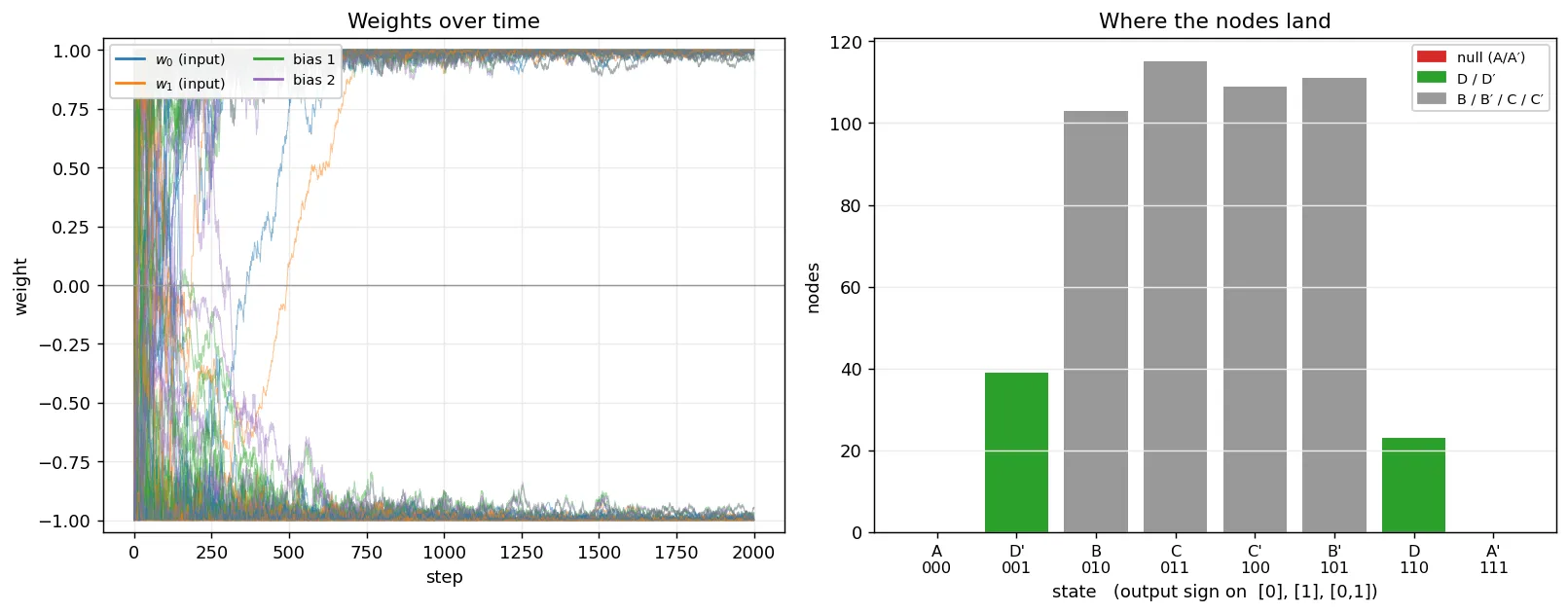
Now D and D’ both appear. Two biases together carry enough weight to tip the combined read in either direction, so the node finally reaches the off-origin states, and it reaches both the state and its anti-state. Their basins are small, but they are no longer empty.

The bias magnitude#

What sets how far the bias can move the boundary is its magnitude — the same magnitude that was inertia and evidence back in Chapter 3b. More conductance behind the bias, more it can outweigh the inputs, and the further off the origin the line can sit. Raise the initialization magnitude and run it again.

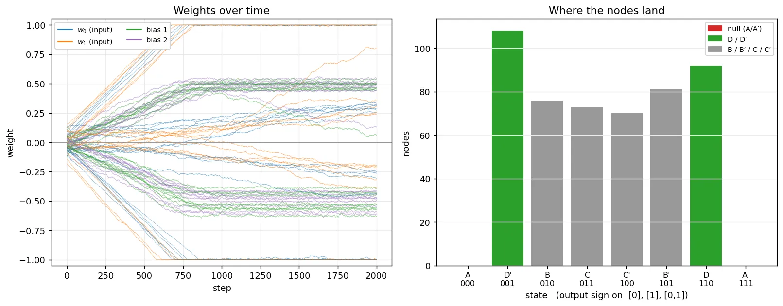
The D and D’ basins fill out, and the six non-null states settle into a balanced set with the null gone. With enough magnitude behind the bias, the node reaches the whole landscape that the bias-free version had locked away.

Telling one attractor from another#

We have been reading a node’s state straight off a weight-space plot, but that only works for two synapses, where two weights make a picture you can draw. The bias nodes already broke it: a node with three or four synapses has a weight on every axis, but we can only draw two. We need a way to name a state that does not depend on drawing the weights at all.

So lets watch what the node does. A node’s whole job is to answer: hand it a pattern, run an FF read, and it says positive + or negative −. Two nodes that give the same answer to every pattern are the same node as far as anything downstream can tell, whatever their exact conductances happen to be. Name a state by its answers. Run the node to convergence, then quietly probe it with each input pattern in turn — a low-voltage read that reports the sign without nudging the weights — and write the signs down in order:

fingerprint = tuple(int(np.sign(lane.evaluate(p, "FFLV"))) for p in patterns)

That tuple is the state’s name. Read the signs as bits, + for 1 and − for 0, and the name is just a number. It works the same for two synapses or two hundred.

Try it on the four-corner node we already understand. That node sees two patterns, [0] and [1], so its fingerprint is two signs — a two-bit number with exactly four values. Those four values are the four corners from the first plot.

Size up the attractor basins#

With a name for every state, two questions that were impossible to answer from a smear of dots become a matter of bookkeeping. How many distinct states does a node settle into? Seed a few hundred of them at random, run the unsupervised cycle, fingerprint each one, and count the distinct numbers that come back. How big is each basin — how much of the random starting ground drains into a given state? Count how many of the seeds land on each number. One histogram answers both: the number of bars is the number of attractors, and the height of each bar is the size of its basin.

Three ways to wire the same two bits#

An encoding maps our input states to distinct AATs, and we can do that in many ways. We have been using one without naming it. Here are three of them for the same two binary inputs, ordered from the most synapse sharing to the least.

The overlapping encoding is the two-synapse node we have been running. Both bits draw on the same two synapses, and there is no address for nothing, so (0,0) cannot even be expressed — three active patterns over two shared synapses.

The two-hot, or dual-rail, encoding gives each bit its own pair of addresses, a 0-line and a 1-line, and the value of the bit picks which one fires. Two bits become two address spaces of two channels each, the AAT is just (x0, x1), and a zero is no longer the absence of an input — it is a channel that lights up and gets reinforced like any other. All four inputs, (0,0) included, are real signals now.

The one-hot encoding goes all the way to no sharing: each of the four whole input combinations gets its own synapse, in a single space of four. No two inputs ever touch the same device.

Run a few hundred random nodes under each map and fingerprint where they land. No biases this time — just the input synapses, so what we are watching is the encoding alone.

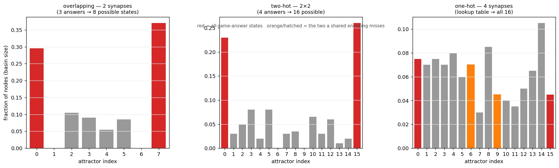
Read across the three panels, all run with no bias. Overlapping is the null collapse from before: about two-thirds of the nodes pile into the two all-same-answer states, and several states never form. Two-hot eases that to about half and spreads the rest over many more states. One-hot has no sharing left at all: each input owns its own synapse, so the node is just a lookup table and every entry settles independently. The flat landscape is no surprise — every state fills, the all-same-answer basins shrink to a sliver, and the node reaches as many distinct attractors as the inputs allow.

So the AAT patterns you push through a lane, worked on by unsupervised AHaH plasticity, set the whole landscape of attractors: which states exist, how big their basins are, how stable each one is. Change the encoding and the landscape moves, sometimes drastically. Add an RA bias and it moves again.

Picture a river. Water flowing over the structure of the riverbed takes on structure of its own — the standing waves and the eddies trace the bed beneath them. The AATs flowing through a neural lane do the same thing to the weights: the input stream presses a mirror of itself into the conductances, and that structure then decides how the node answers the stream. The data shapes the kT-bits, and the kT-bits shape how the data is read.

Which raises the obvious question. We have counted these states and measured their basins, but we have not said what a single one of them is for. What is a node sitting in state B actually doing?

Unsupervised AHaH attractor states are logic functions#

Look again at our fingerprint. It is the sign of the output for every input pattern, written in order. That is a truth table. The number we have been using to tell one attractor from another is the same number an engineer would use to name a two-input logic gate.

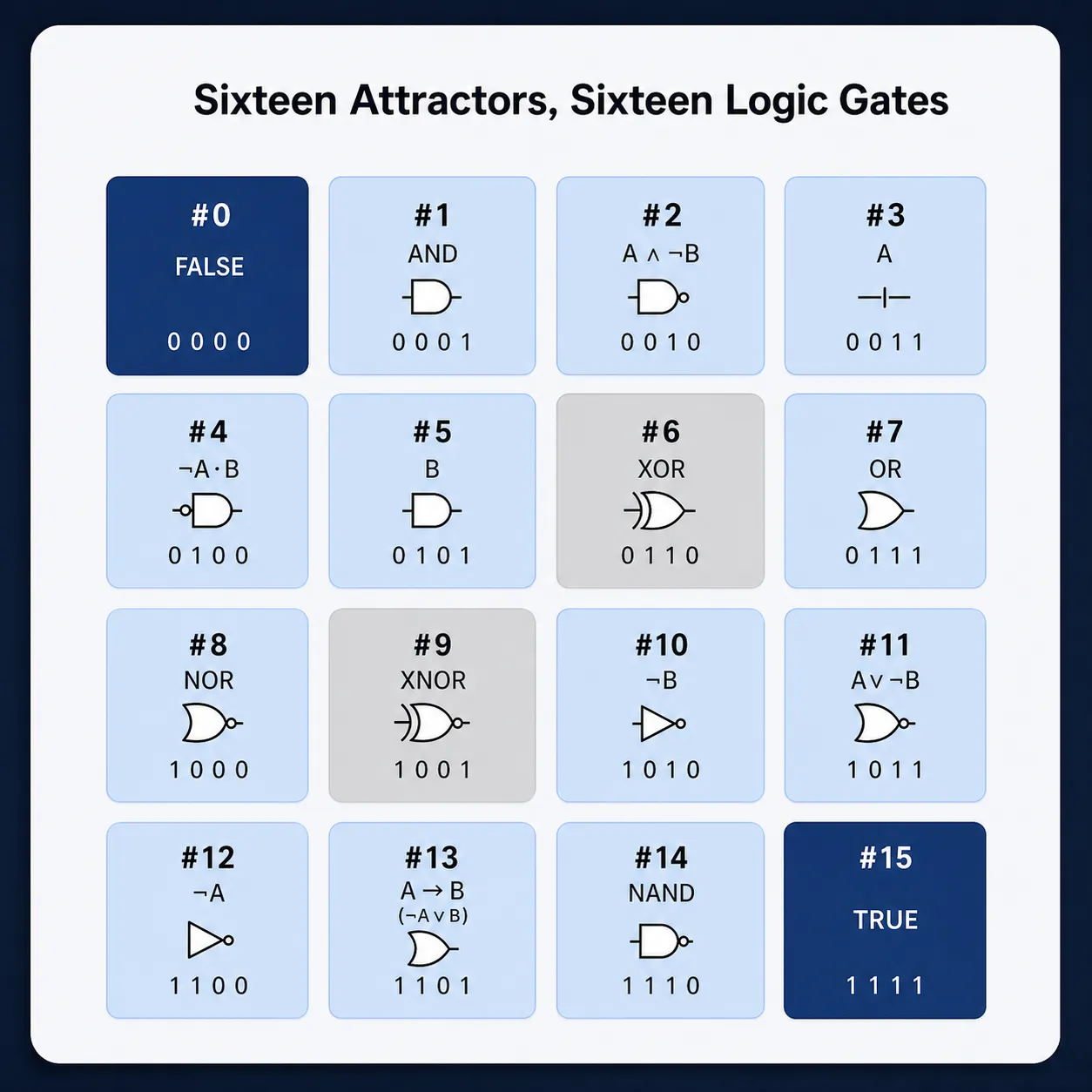
The two questions from the histogram now answer themselves. The two giant basins (without the RA bias’) are the constant gates — always-false and always-true, the same answer to every input—what we call the ‘null’ states. They are the laziest thing a Hebbian node can do and the most stable once it gets there, which is why so much of the random ground drains into them. The two states that a shared encoding never reaches are XOR and XNOR. With two synapses and a bias, the output is

and the decision boundary — where the node flips from + to − — is the line $y = 0$. The weights tilt that line and the bias slides it around the plane, but it stays a line; nothing here can bend it. A straight line, wherever you put it, splits AND from the rest, or OR, or any of fourteen of the gates. It cannot split XOR: XOR puts opposite corners of the input square in the same class, and no straight line ever does that, bias or no bias. XOR is not missing because the bias is absent or the learning rule is weak. It is missing because a single node draws a straight line, and XOR is not linearly separable.

Give every input its own synapse and the four inputs become four independent axes, and across those axes every one of the sixteen functions is linearly separable, XOR and XNOR included. The encoding is what made them separable, not the node — the node is still drawing a single straight cut, it just does it in a space where one cut suffices.

So: an AHaH attractor state is a logic function. A node settles into one with nobody supervising it, the function it lands on is set by its random start and the data it sees, and the encoding decides which functions are on the table at all.

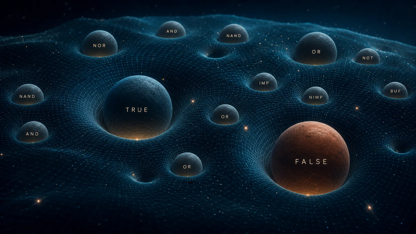
Trace that back to the single kT-bit and the moves are simple. Hebbian feedback locks a pair into a sign and holds it there. Anti-Hebbian feedback does the opposite: it unlocks the pair and drives it back toward the indeterminate middle. Lock and unlock. Put several pairs on a shared lane, feed them structured input data, and they fall into an attractor that is a logic function of the input.

Think about it! Nothing in the lane was ever told what a logic gate is. The gate assembles itself, and the blueprint for it is the structure of the data. The data carries the information for its own logic gates — the information for self assembly is in the datastream.

The path less traveled, how deep does it go?#

The next few chapters turn practical. We are going to build a pipeline that assimilates transformer architectures onto kT-RAM, and to get there we lean hard on supervised classifiers built on kT-RAM and set the thermodynamics off to the side. The read voltages go up, and the substrate starts to look like ordinary deterministic learning. That is a choice about how we run it. The substrate underneath has not changed. Turn the read voltage back down and the thermodynamics comes right back — the node stops settling on one answer and starts drawing thermal samples again, the way a kT-bit read at low voltage did in Chapter 3b.

That read voltage is a door, and we are about to walk (temporarily) past it. Before we do, I want to leave it open for you, because a fundamentally new world lives behind that door.

In the next chapters I am going to show you one path through this territory, one that is aligned most strongly with the current AI hype train, but it is just one path. The space of architectures you could build out of these nodes runs vastly broader and deeper than anything I will reach, and it is wide open — almost none of it has been tried. You could spend a lifetime in here and not find the edges.

If any of this has caught your attention, go exploring. I would love to hear what you find!

Next: Chapter 5b: AHaH Attractors → A Battle for the Margin