Chapter 3b: The Thermodynamic Bit, Derived

Every weight in a neural network is a single number — usually a float A floating-point number — the standard way a computer stores a real value like 0.732, in a fixed number of bits. , sometimes a quantized int, but always one value N bits wide. That single number is what learning algorithms exist to adjust — train a model and you are tuning billions of them. A differential synapse does that job with two memristors A memristor is a resistor with memory: how easily it passes current depends on its history. That lets one device store a value, not only carry one. instead. Their balance acts as the weight, but the pair holds more than any single number can. We call that pair a kT-bit, and when used in the context of neural networks it plays the role of a synapse. It may seem like a small change, but a lot of what we normally engineer into a learning system comes free with it, written into the physics rather than the code.

A kT-bit is built from two memristors#

A memristor is a resistor with memory: put a voltage exceeding its threshold across it and its conductance changes. We draw it as an hourglass/infinity symbol with a stripe on one end, and that stripe is the cathode. Drive current into the cathode and the conductance climbs; reverse and it falls. A short positive pulse leaves the device a little more conductive, a short negative pulse walks it back.

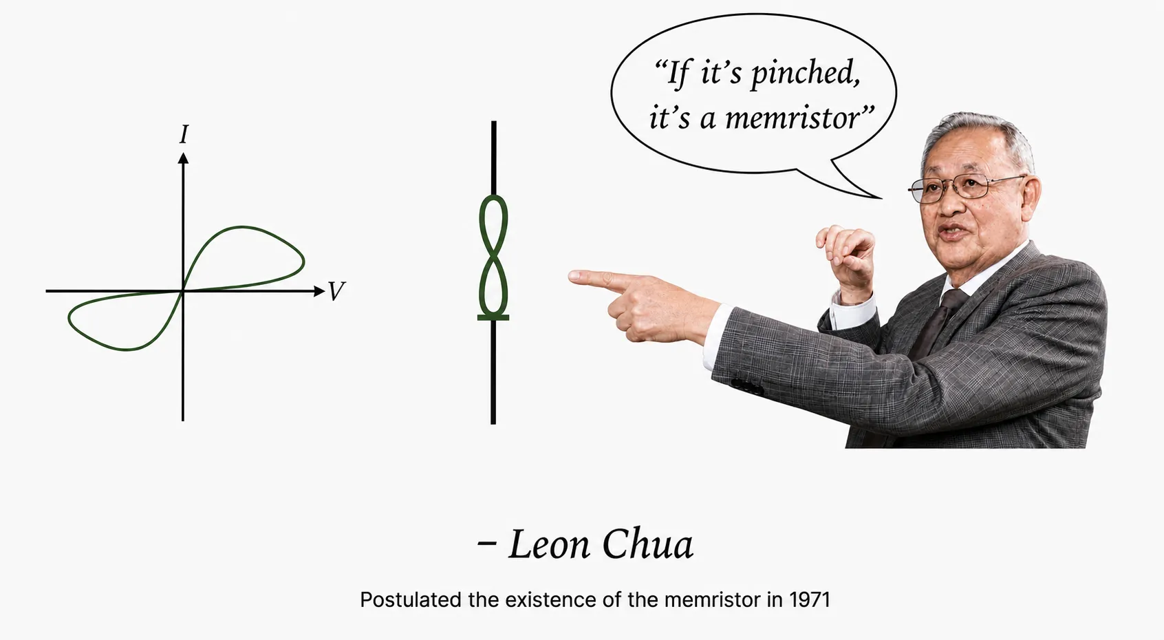
The infinity is easier to draw by hand than the standard symbol, but it also points straight at the one property that defines the device. Put a slow sine wave across a memristor and plot current against voltage and you do not get a straight line — you get a loop pinched shut at the origin. Leon Chua, who named the memristor in 1971, put it plainly: if it’s pinched, it’s a memristor Chua also drew a symbol for it: a square wave inside a rectangle, with a bar marking polarity. The trouble is the bar runs opposite to essentially every other electrical convention, where the cathode is the negative, lower-potential end. He’s an impressive guy, but the symbol is objectively poor. Its hard to draw and bears no symbolic relationship with the defining characteristic of a memristor. So we fixed it.

Two memristors make a voltage divider#

You can wire two memristors into a kT-bit a few different ways. The one we show here is the 2-1 “series voltage divider”. Stack the two devices in series, and read the junction between them.

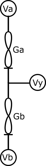
Drive the top at +V and the bottom at −V, measure the voltage at the junction between the two devices, and that junction voltage Vy reports the balance of the two conductances:

The read voltage V is not fixed — turning it down is how you slow the adaptation or quiet a read — so the output is reported normalized by V, a unit-less value y = Vy / V that lands in [−1, 1] no matter how hard you drove the pair. That y is what every read returns.

That is the entire circuit. What makes it compute is how you drive it, and the drive is the kT-RAM instruction set. Every instruction is a two-letter code: the first letter sets the voltage direction across the pair — F for forward, R for reverse — and the second letter sets what happens at the y node. Float it and you read the pair; lock it to a feedback voltage and you nudge the two conductances one way or the other. Reads report y; feedbacks move it. The full table is in the cheat sheet at the bottom of this page, and you can drive a live pair with the simulator there — for the rest of this article, that two-letter pattern, a voltage direction and a feedback, is all the control you need.

The open-source Neural-Lane Emulator gives us a simple simulator and the instruction set to drive it. Set the spaces-per-lane and the lane count to one and the lane collapses to one device on each side, selected by the fixed AAT z = (0,) — the entire API surface this needs. A differential pair is not a traditional single-number weight. It carries an extra dimension, literally, and that dimension changes how the weight works and what it can do.

from ktram_neural_core import Core

core = Core(1, 1, spaces_per_lane=1, num_lanes=1,
            model="float", init="medium", seed=1)
lane = core.lane(0)
z = (0,)                        # the AAT: address 0, the one space

y      = lane.evaluate(z, "FF") # forward read -> the weight, in [-1, 1]
ga, gb = core.read_gab(0, z)    # peek at the two conductances (debug/emulator only)

Everything below runs on the Float device, the cleanest of the four. With that one synapse in hand, here is what it carries that a float cannot.

One synapse, two conductances#

Read one or more pairs and you get one number back, the neural activity value y. In reference to a single kT-bit, we call that value the weight w.

A differential pair has two “modes”. The differential mode is the difference between the conductances Conductance is how easily current flows through a device, the inverse of resistance. Higher conductance means more current for the same voltage. , Ga − Gb. The common mode is their sum, Ga + Gb. The weight is the first divided by the second:

A single floating point number is also just one number, so you may be thinking that the differential pair just looks like an expensive way to store a float. First, two memristors is still quite a bit less hardware real-estate than, say, 16 SRAM cells Static RAM, the fast on-chip memory that holds digital bits. A standard SRAM cell is six transistors and stores one bit, so a 16-bit weight takes 16 × 6 = 96 transistors, against the two memristors here. . Second, the pair holds a hidden property that changes the game. Double both conductances of the pair and the weight does not change, so a read tells you the balance between the two and not the total. That total is the second number, the magnitude, or common mode:

A conventional weight gives you just a single number. A pair gives you two numbers, and the way that they interact hides some truly remarkable properties that are foundational for learning and inference.

Magnitude growth anneals the weight#

A feedback instruction One of the active two-letter codes (FH, RL, FU, …) that nudges the two conductances up or down — as opposed to a read, which only reports y. See the instruction cheat sheet at the bottom of this page. moves the conductances by a fixed amount, but the weight does not move by an incremental amount, because the weight is normalized by the magnitude. Push a conductance by a fixed step and the weight shifts by that step divided by m. Big magnitude, small shift; small magnitude, big shift. The magnitude is the weight’s inertia — how hard it is to move.

Let’s run an experiment: set two pairs to the same starting weight but different magnitude, then drive them identically. set_start_y(..., level=) scales the magnitude directly — m = 2 · level · GMax — so you get a matched weight but a mismatched magnitude.

z = (0,)
mk = lambda: Core(1, 1, spaces_per_lane=1, num_lanes=1,
                  model="float", init="medium", seed=1)
young, mature = mk(), mk()

young.set_start_y(0, z, y0=0.3, level=0.05)   # small Ga+Gb
mature.set_start_y(0, z, y0=0.3, level=0.5)   # 10x the magnitude, same starting weight

# drive both with the identical (FF, RH) stream and record w each step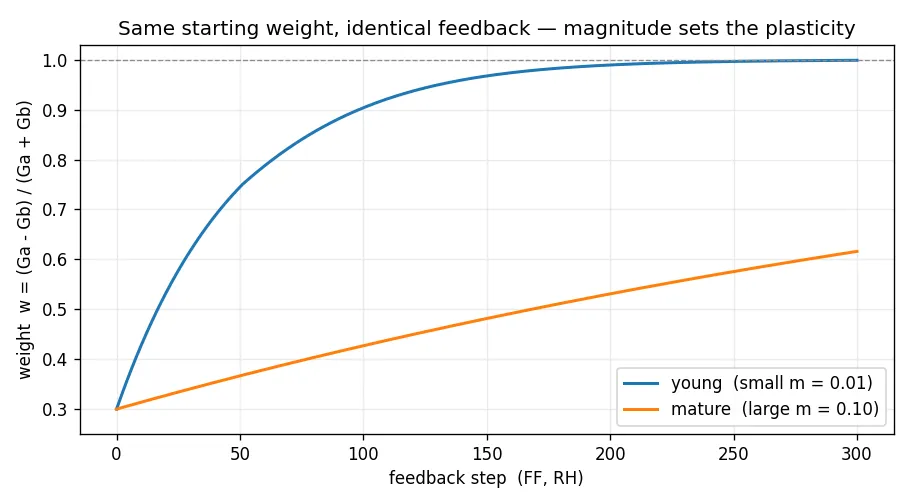

Same starting weight, the same feedback into both, and the low-magnitude pair commits ten times faster. Nothing scheduled that rate — the magnitude set it, because the magnitude is in the denominator.

This is annealing Take big learning steps early and smaller ones as you go, so you settle into a good answer instead of bouncing around it forever. The word comes from metalworking: cool the metal slowly and it finds a calmer, lower-energy arrangement. , baked into the physics of a differential pair. A synapse’s magnitude grows with use, so it slows its own learning as it goes — big steps when little is behind it, small steps once a lot is. Machine learning buys the same curve by hand, tuning a schedule that shrinks the step as training proceeds. Here no one writes the schedule: the magnitude is the annealing schedule, and it comes free from the physics. A float has none of this, which is why almost every ML training pipeline includes an annealing schedule.

The magnitude is a count of evidence#

Read the same two numbers a second way. Forget conductance for a moment and call the a-side and the b-side two running tallies — votes for “positive” and votes for “negative.” The magnitude m = Ga + Gb is the number of votes cast. The weight w is not that count, and it is not the raw lead of one side over the other either — the raw lead (or ‘lean’) is the differential mode, Ga − Gb. The weight is that lead divided by the total: the share of the vote, how far the tally leans, in [−1, 1]. Three positive out of four leans exactly as far as seven hundred and fifty out of a thousand — same w = 0.5. But the second rests on two hundred and fifty times the votes. The lean is identical; the evidence behind it is not, and m is what tells a hunch from a conviction.

You can build such a tally with the instruction set directly, and the kT-RAM instruction that grows the count is the forward feedback. FH adds a quantum to Ga — a vote for the positive side; FL adds one to Gb — a vote for the negative. Each touches one side and only adds, so the magnitude m = Ga + Gb is the literal number of votes cast. The reverse feedbacks RH and RL move the weight the same directions but by lowering the opposite conductance, which depletes the pair rather than accumulating it — a leaky average instead of a count.

This is the inertia from the last section wearing its second hat. More evidence means a larger magnitude, and a larger magnitude is harder for any single feedback to move. Probabilistic confidence and inertia are the same number: a synapse that has seen a lot is both sure and slow to change its mind.

There is a clean statistical reading of this, and it borrows two terms from Bayesian statistics. The two conductances behave like the parameters of a Beta distribution Picture a dial that guesses “how likely is yes?” At first the guess is fuzzy and spread out. Each new yes or no nudges it and sharpens it. That whole curve of guesses, fuzzy or sharp, is the Beta distribution. , the standard way to describe a belief about a yes-or-no probability you are still learning, like the bias of a coin. A Beta is built from two pseudo-counts Two running tallies: how many times you have seen “yes” and how many times “no.” They are called pseudo-counts only because the math lets them be fractional instead of whole numbers. : how many times you have seen “yes” and how many times “no.” (Pseudo because they need not be whole numbers.) Map Ga to the yes-count and Gb to the no-count, and both of our readings fall straight out of it.

The distribution’s mean says where the belief sits, which way it leans, and that is the weight w (rescaled to [−1, 1]). Its concentration How tall and narrow the belief curve is. As evidence piles up the curve concentrates into a sharper spike, which is another way of saying you are more certain. is the sum of the two counts, Ga + Gb, which is exactly the magnitude m. Concentration is the total weight of evidence, and it sets how peaked the curve is. A few counts give a broad, uncertain hump. Many counts give a narrow spike over the mean. Turn the concentration up and the variance falls roughly as its inverse: more evidence, less spread, more certainty.

So the pair holds a belief: The number is the weight w. How sure it is of it is the magnitude m. A float keeps the first and throws the second away.

What evidence buys you when pairs combine#

The payoff arrives when you read more than one pair at once. A neural lane couples its pairs into a single 2-1 divider, and by Kirchhoff the junction voltage is the total differential mode over the total common mode — every selected pair’s conductances summed on each side:

Now substitute what each pair already carries. For pair i, the common mode is its magnitude, and the differential mode is its weight times that magnitude:

The second equation is just the single-pair definition $w_i = (G_{a,i} - G_{b,i}) / m_i$ rearranged. Put both into the divider and the bare conductances drop out, leaving only each pair’s weight and magnitude:

That is a magnitude-weighted average of the individual weights. Each synapse votes with its weight $w_i$, and its vote counts in proportion to its magnitude $m_i$ — its evidence. A confident pair dominates the result; an unsure one barely registers. No code arbitrates between them; the divider does it by physics.

Combining estimates in proportion to available evidence is what Bayesian inference Reasoning with probability: hold a belief, then revise it by a fixed rule (Bayes’ theorem) each time evidence arrives. The more evidence, the less your starting guess matters. does when it pools independent observations. The same passive structure we picked for its normalized output now doubles as an evidence-combiner. That resemblance is strong enough to test rather than admire.

Is the differential pair really Bayesian?#

Recall the Beta reading from the last section: the two conductances act as the pseudo-counts of a Beta distribution, $\alpha = G_a$ for the “yes” tally and $\beta = G_b$ for the “no.” Three summary numbers come off that distribution — its mean, its concentration, and its variance:

The pair’s two readings are the first two, renamed:

That much is algebra — true by substitution, whatever the devices do. The real question is whether the dynamics follow Bayes, or only the labels match. Three steps settle it: a vote is a tally, Bayes pools tallies by adding, and Kirchhoff adds.

Step one — a vote is a tally. The Beta is the natural belief here because of conjugacy A lucky property: after you fold in a new observation, your belief keeps the exact same shape it had before, with only the tallies changed. So updating your belief is nothing more than adding one to a count. : observe one more yes-or-no sample and the posterior Your belief after seeing the data, as opposed to the prior — your belief before any data arrived. is another Beta with a single count bumped.

That is what forward feedback does. FH adds a fixed quantum $\delta$ to the a-side and leaves the b-side alone; FL mirrors it. After $n_+$ and $n_-$ votes the conductances are $G_a = G_a^0 + \delta\, n_+$ and $G_b = G_b^0 + \delta\, n_-$ — term for term the Beta posteriors grown from the initialization, the prior. (Reverse feedback RH/RL reaches the same weights by lowering the opposite side, so it never grows the count: a leaky average, not the conjugate update.)

Step two — Bayes pools tallies by adding them. Independent yes/no evidence about the same unknown probability combines by summing the counts: $\text{Beta}(\alpha_1,\beta_1)$ and $\text{Beta}(\alpha_2,\beta_2)$ pool into $\text{Beta}(\alpha_1+\alpha_2,\ \beta_1+\beta_2)$. Conjugate updating is score-keeping, and combining scorekeepers is adding their scores.

Step three — Kirchhoff does the addition. Parallel conductances sum — that is Kirchhoff’s current law When several wires meet at a junction, the currents flowing in simply add up. Nobody keeps the books — the physics does the sum on its own. , the same fact behind the lane equation above. The pooled mean from step two, rescaled to $[-1,1]$, regroups into exactly the lane output:

No code runs anywhere: the addition Bayes asks for and the addition the wire performs are the same addition. The junction voltage is the mean of the count-pooled posterior; the pooled confidence $\sum_i m_i$ rides in the total current, a separate read.

Caveats. Two limits, both common sense. First, it depends how you use the lane. The pooling is a true Bayesian combination only when the pairs hold independent evidence about the same probability, like a redundant sensing lane. Wire the same pairs into a classifier or a logic gate and the arithmetic is identical, but “pooled posterior” becomes just an analogy. Second, the devices are analog and physical: a conductance saturates where a Beta count would climb forever, so the exact tally holds only before a pair rails.

Step back from the caveats. The annealing schedule fell out of the pair for free — no one wrote it, the magnitude was it — and probabilistic inference falls out the same way. We did not build a Bayesian update or a pooling rule; we wired two counters to a wire, and the voltage at the junction came out as the mean of a pooled Bayesian posterior. The edge cases are real, but they do not dim the main fact: a kT-bit does Bayesian inference because of what it is, not because of anything we programmed into it.

Low-voltage reading is probabilistic sampling#

Up to now every read came back as a clean number, the exact ratio of two conductances. Real reads aren’t clean. A memristor is a physical device, and physical devices hiss. Two sources set the hiss. There is thermal Johnson–Nyquist noise — the hiss you hear in an amplifier turned up with nothing playing, fixed by temperature. And there is 1/f flicker and random-telegraph noise, the conductance wandering as charge traps fill and empty, which in a real memristor is the louder of the two. The hiss is unavoidable. Account for it and yet another result falls straight out of the physics.

So the question is how loud the hiss is, and how its loudness moves.

Both come out of the physics device by device, and the full derivation — Johnson’s law on the junction resistance, the fractional-fluctuation algebra that drops the (1 − w²) factor out of the ratio, and how the two combine — is on a companion page. Here are just the results. The thermal term rides on the junction resistance 1/m, so it falls as the pair grows; and because we read y = Vy / V The output voltage at the junction, Vy, is normalized by the read voltage V that drove the pair, which is what puts the weight y on the same [-1, 1] scale regardless of how hard you read. , a gentler read lifts it as 1/V. The flicker term is the conductances wandering by a fixed fraction of themselves; push that fraction through w = (Ga − Gb)/(Ga + Gb) and a (1 − w²) factor falls out — widest when the pair is balanced, closing to zero as either side takes over — while the fraction itself shrinks with evidence as 1/√m. Thermal noise does not care how hard you read; flicker carries no factor of V at all. The two add in quadrature:

So a read does not come back clean. It comes back as the weight plus a kick of noise: a sample scattered around what the pair believes. And the width of that scatter tracks the belief. Both terms fall as 1/√m, so a pair that has seen little reads loud and a pair that has seen a lot reads quiet — the same m that set the inertia and counted the evidence. The flicker term adds the second half: its (1 − w²) is widest at the balance point and closes toward the rails, so a pair that has made up its mind reads tight.

That is the shape of the Beta posterior from a few sections back. Line up the variables and the match is plain: the magnitude m is the Beta’s concentration $\kappa$, the weight w is its mean $\mu$ rescaled, and $\mu(1-\mu) = (1 - w^2)/4$. So the Beta’s variance $\sigma^2 = \mu(1-\mu)/(\kappa+1)$ narrows the same two ways the read does — with evidence as m climbs, and toward the certain ends where the $(1 - w^2)$ collapses. (The companion page lines the two up term by term.) The device’s read scatters the way its belief is spread. Nobody programmed that match. It is one more thing that pops out of the physics: the device samples its own posterior, and the randomness is the device’s own noise — no pseudo-random algorithm, no code drawing the sample. The kT-bit is the random number generator.

That is Thompson sampling A classic strategy for acting under uncertainty: instead of always picking the option that looks best on average, you draw a random sample from your current belief about each option and act on the draw. When you are unsure the samples are spread out, so you naturally try different things; as evidence sharpens the belief, the samples concentrate and you settle on the winner. , in a single read. The best way we know to act under uncertainty is to draw from your belief and commit to the draw: unsure, the draws spread and you explore; certain, they collapse onto the answer and you exploit. Software buys this with a stored variance, a random-number generator, and a schedule to cool the exploration as the belief sharpens. Here the magnitude is all three at once. A confident pair commits, an unsure pair explores, and the search cools itself as evidence comes in. Nothing schedules it. The explore-exploit loop at the center of every agent that learns by acting is a property of the kT-bit.

How far does the match run? The shape is free and always there: both terms fall as 1/√m, and the flicker term carries the (1 − w²) that closes toward the rails, so the read’s spread tracks the belief’s across the pair’s whole range. What you can still set is how high the thermal term rides above the flicker floor, with the read voltage V — the thermal term goes as 1/V, so a gentler read lifts the hiss while the flicker floor itself stays put. Confidence-proportional sampling is the physics; the read voltage is the one knob that sets how far above the floor you read — the read-voltage slider in the simulator below.

The magnitude was the inertia, then the count of evidence, and now it sets how loud the read is: a pair that has seen a lot reads quietly, a pair that has seen little reads loud. Sure and quiet are one condition, unsure and noisy another, and m sets both.

And the read voltage is a knob you can turn. Raise V and the read sharpens toward the flicker floor; drop V and the thermal hiss climbs above it — σ_thermal ∝ 1/V, a dial on how far above the floor you sample. The low-voltage reads FFLV/RFLV already sit well below the switching threshold, so they report the pair without disturbing it. Put those together and one voltage buys you two things at once: you read a synapse without changing what it knows, and you set how widely it samples while you do it — no extra circuitry, no stored temperature, just V. The read-voltage dial in the simulator at the bottom of this page is exactly this knob: pick a low-voltage read (FFLV/RFLV) in free play and slide it down to push V further below threshold — the weight line holds still while the scatter around it widens.

Try the coin flip in the simulator below. Drive the pair to its balance point and the clean weight is zero, so the read is pure hiss, its sign as likely up as down. Hold down a Hebbian read from there and the first noisy sample tips the pair, and the positive feedback runs with it to a rail. Reset, run it again, and the other rail comes up just as often. A fair coin, pulled straight out of the device’s own noise. Lean the pair before you let it run and the hiss has to overcome a head start: the coin comes up biased, and the bias is the weight you stored — a random bit you can write. That one is worth its own chapter, and it is coming.

In a nutshell: reading the pair never returns a clean number; it returns a noisy draw centered on the stored weight, and the sign of a single read is a random bit that falls on the weight’s side more reliably the bigger the weight is next to the noise. Two things set that noise: how much evidence the pair has gathered, which quiets the reads on its own, and how gently you read it — drop the read voltage and the noise grows, with the stored weight left untouched. So the same pair read at full strength gives its best answer, and read gently gives a random sample of what it believes — you choose which, just by how hard you read.

And that’s not all#

Once you see that a kT-bit or differential synapse is a running tally read as a ratio, the matches come fast.

Robbins–Monro. From optimization theory: home in on an answer from noisy samples by taking steps that shrink as 1/n. It comes with a proof that this shrinking-step average actually converges. That per-vote update, $\Delta w = \delta(1-w)/(m+\delta)$, is the running-average rule — the same $\Delta\mu = (x-\mu)/n$ every student computes for a mean, with the magnitude $m$ standing in for the count $n$. That $1/n$ step is the schedule from stochastic approximation that carries a convergence theorem: steps that sum to infinity while their squares stay finite. The pair does not just anneal on some schedule — it anneals on the schedule the theory proves will converge, with no one choosing it.

Precision Weighting. From statistics and signal processing: when you combine several noisy estimates, weight each by its precision (how sure it is) instead of equally. Confident sources count for more. The lane’s pooling has a name too. Giving each pair a say in proportion to its magnitude gives it a say in proportion to its precision, since the variance goes as $1/m$ — and that is how a Kalman filter fuses sensors and a meta-analysis pools studies. The equation an engineer knows as sensor fusion is the equation a statistician knows as pooling a posterior, and the wire runs both.

Common-Mode Rejection. An electronics term: a differential circuit responds to the difference between its two inputs and ignores whatever moves both together, like noise, drift, or temperature. This is the reason differential pairs sit at the input of nearly every analog chip ever drawn. Anything that pushes both conductances together — temperature, supply drift, the slow aging that touches both devices alike — cancels in the ratio. The belief is held as a balance, so it shrugs off the drift that wrecks single-device analog memory. We did not add that; it is the differential form, free, the way circuit designers have always gotten it.

Drift-Diffusion Model. From cognitive science: the standard account of a two-choice decision. Evidence accumulates noisily until it crosses a threshold, and that is the moment of choice. Read $G_a - G_b$ as evidence piling toward a threshold and you have the standard account of how brains settle a two-way decision, with the rails as the bound — saturation stops being a defect and becomes the moment the synapse makes up its mind.

Opponent Coding. From neuroscience: representing a value as a tug-of-war between two opposing channels (on vs. off, red vs. green) rather than one signed number. Nature keeps reaching for the same trick: ON/OFF cells in the retina, opponent color channels, excitation balanced against inhibition. Two counters in tension, chosen again and again over a single signed number.

Would you look at what keeps falling out of two memristors and a wire!

Still here? Get to know the kT-RAM instruction set#

The article could have ended a paragraph ago. Annealing, Bayes, and a half-dozen other names all fell out of two numbers and a wire. But if you are still reading, you are probably the kind of person who now wants the actual controls: the two-letter codes that drive the pair. The cheat sheet and live simulator are right here — and what follows them is the quick tour, one picture per instruction family. Every plot is a cell in the companion notebook: change a string, rerun, watch the two numbers move.

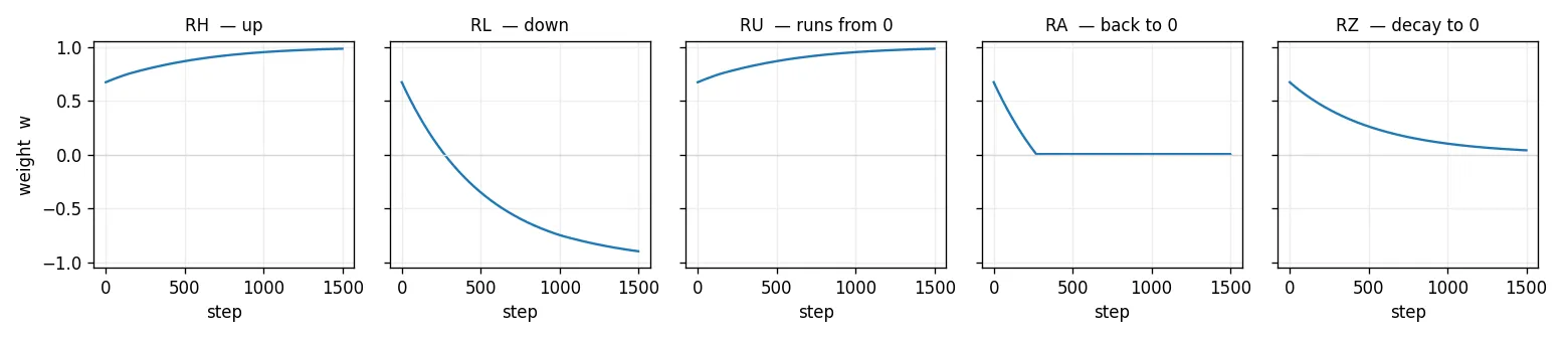
The feedback instructions, side by side. Nudge a pair to a clear positive lean, then repeat one feedback and watch where it goes. RH drives up, RL down; RU runs away from zero and RA snaps back toward it (the two unsupervised moves); RZ decays the lean to zero. The forward set (FH, FL, FU, FA, FZ) mirrors all five.

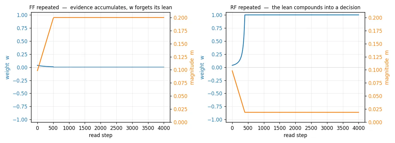
Which read you repeat picks the outcome. With no feedback at all — just the same read over and over — FF is anti-Hebbian Hebbian learning is the neuroscience rule “neurons that fire together wire together”: co-activity strengthens a connection. Anti-Hebbian is the reverse, weakening it and spreading activity out instead of concentrating it. : it piles evidence onto both sides, so the magnitude m grows while the lean w washes to zero. RF is Hebbian: the lean compounds until the pair commits to a rail. Same pair, opposite fate, set by which read you hold down.

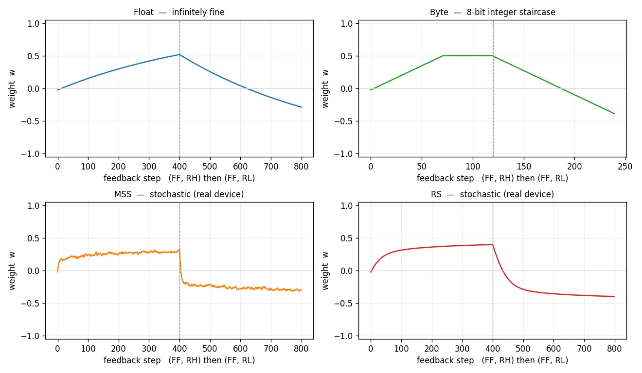
The same drive on four devices. The identical pulse — (FF, RH) up to a plateau, then (FF, RL) back down — runs on infinitely-fine Float, on the 8-bit Byte (an integer staircase that tops out at the quantization ceiling Quantization rounds a smooth value onto a discrete ladder of steps. With 8 bits there are 256 rungs, so the value can’t be finer than one rung and can’t climb past the top rung, the ceiling. ), and on MSS and RS, the real stochastic physics of a Knowm device. Same lesson on each; the model only sets resolution and noise.

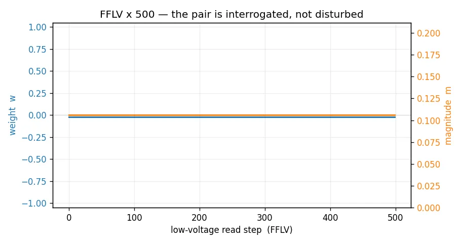
Reading without disturbing. A normal FF read drives the devices at full voltage, nudging the state a little every time. The low-voltage read FFLV drops below the threshold, and for Float and Byte the sub-threshold dead-zone makes that disturbance exactly zero — you can ask a pair for its weight and magnitude without casting a single vote.

Two memristors and a wire. We did not program the inertia, the annealing, the Bayesian belief, or the coin pulled straight from kT — every one of them fell out of the balance of two conductances and the way a wire adds current.

Next: Chapter 3c: The Thermodynamic Bit, Built