Chapter 6: Classification and Thermal Sampling on kT-RAM Neural Lanes

At the end of Chapter 5b I said the next move was to hand the lane an answer key. So let’s do the simplest supervised thing there is: show it labelled examples and have it learn to name them.

The task is Iris, the “hello, world” of classifier tasks. It is a small table of measurements the statistician Ronald Fisher published in 1936, and people have been testing classifiers on it ever since. It holds a hundred and fifty flowers, fifty from each of three iris species: setosa, versicolor, and virginica. Every flower carries four numbers in centimeters — the length and the width of a petal, and the same two for a sepal, the green leaf-like part beneath the petals. The species is the label. The job is to read the four numbers and name the flower. It is small enough to plot on one page and read with your own eyes.

We are going to turn the raw measurements into AATs, feed them into a stack of neural lanes, and train those lanes with a kT-RAM instruction-set routine that gets us logistic regression.

pip install "git+https://github.com/knowm/ktram-neural-core.git#subdirectory=python"

The code example is in examples/iris-classifier in the repo. The whole chapter also runs as a workbook you can open in Colab and poke at, covering the encoders, the three-case rule at L0, RankCut, the benchmark, the hot reads, and the chained-against-synchronous sampler:

One lane per label#

A single neural lane draws one linear cut through its inputs and answers positive (+) or negative (−). One cut sorts the world into two piles, which is enough for is this a setosa or not, but the Iris dataset has three species. So we use three lanes, one per class, and ask each the yes-or-no question it can actually answer:

• lane 0 — is this a setosa?
• lane 1 — is this a versicolor?
• lane 2 — is this a virginica?

Each lane is its own linear neuron with its own weights, reading the same input. To classify a flower you read all three and take whichever returns the highest voltage.

Encoding data as AATs#

A lane does not read numbers. It reads AATs. So every input has to become one or more address tuples before a lane sees it. We use “AAT Encoders”, or just “Encoders”, to do this.

The encoder interface is small on purpose. An encoder needs two things. encode(value) returns the AAT, one channel index per space. space_sizes says how many channels each space holds, which is what the hardware or emulator needs to provision itself. An adaptive encoder adds a third, encode_adapt(value), which tunes its internal state to the data before encoding. An encoder that does not adapt only ever runs encode.

How data gets turned into AATs is a design choice, and there is no single right answer. It depends on the native data type, the resources you have, and what you are trying to do. We will have a lot more to say about it in future chapters, and the encoder I’m showing here is a ‘toy’ example. Far more powerful methods exist.

Some data is already most of the way there. An AAT is just integers, and plenty of data is already integers — a category id, a pixel value, or a count. You could take such an integer and feed it in as a channel index unchanged. Usually you should not, because a bare index throws away what the number meant. Send 123,456 in as channel 123,456 and the lane learns nothing about its size or its nearness to 123,457. The two land on unrelated synapses that happen to sit side by side. You could bin the number instead, rounding to the nearest hundred, say. Or you could give each decimal digit its own ten-channel space, so 123,457 encodes to the six-entry AAT (1, 2, 3, 4, 5, 7). We don’t need to think too hard about it here. The point is that there is more than one way to skin an AAT.

A floating point number is not an AAT, so we must encode it. There is no synapse number 4.2. To get an AAT from it you can bin it such that the bin index is the channel. Every one of the four Iris measurements is a float, so we will bin the raw data to create AATs before we hand it off to the lanes.

One encoder for this job is the A2DEncoder. The name is analog-to-digital, the same conversion a sensor does when it turns a voltage into a number: it takes a continuous value and reports which bin it landed in, and that bin index is the channel. The name is an analogy. The measurements are already digital numbers, and an AAT is just a different digital encoding of the same information. The encoder is ordinary arithmetic deciding which bin a float belongs to. Each feature gets its own space of bins, sized by a bits knob — bits=3 cuts the range into eight bins.

Fixed bins#

Never let the encoder adapt and the bins stay where they start, an even slicing of [init_min, init_max]:

from ktram_neural_core.encode import A2DEncoder

fixed = A2DEncoder(dims=4, bits=3, init_min=X_tr.min(0), init_max=X_tr.max(0))
# bits=3 -> 8 channels per feature;   encode([5.1, 3.5, 1.4, 0.2]) -> (1, 5, 0, 0)

Eight fixed bins per feature already classify Iris about as well as anything does, because Iris is small and nearly separable A dataset is linearly separable when a straight cut can put every example of one class on one side and everything else on the other. In more than two dimensions the cut is a flat plane, but the idea is the same. Iris is nearly separable: setosa splits off cleanly, and versicolor and virginica overlap enough that a few flowers always land on the wrong side of any straight cut. That leftover overlap is the accuracy ceiling every linear classifier hits. . But even slices spend bins where there is no data. A bin in an empty stretch never fires, and the flowers all pile into the few bins that cover the crowded stretch. On easy data that waste costs nothing. On skewed or clumpy data it costs a lot.

Adaptive bins#

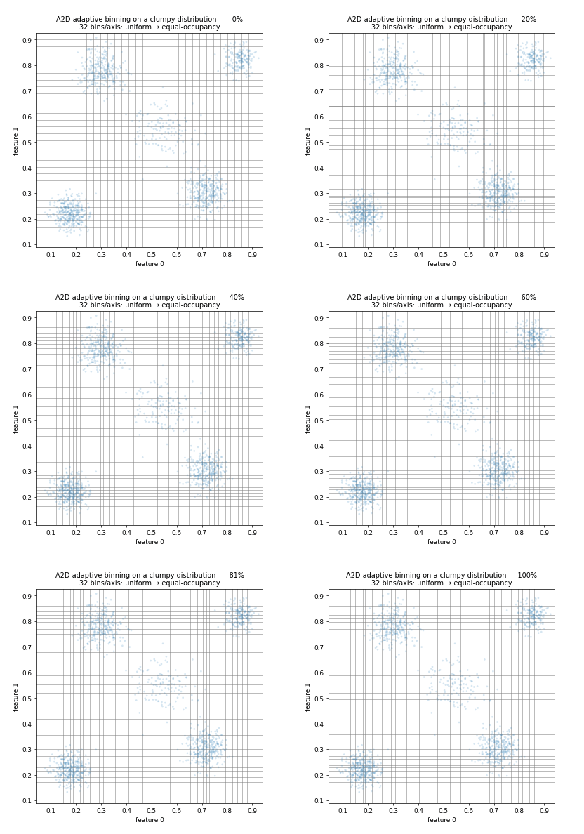
The A2D encoder can also adapt, moving its grid to match the data distribution. Inside it is a binary tree of split points that start at the even slicing and then migrate, every example tugging the nearest edges a little in its direction An exponential moving average: each new value nudges the bin edge a small fraction l of the way toward itself, so the edges drift to wherever the data piles up and stop where it thins out. Set l small and the edges move slowly and smoothly. Set it large and they chase the most recent points. . Where the data crowds, the bins bunch up and get fine. Where it is empty, they stretch and go coarse, until every bin holds about the same number of points — equal-occupancy. The resolution goes where the data is.

It is easiest to see on a made-up two-dimensional spread with a few clumps in it, run at a finer grid than Iris needs. Watch the lines crawl off the empty ground and pack into the clusters:

Run the same thing on the actual Iris measurements:

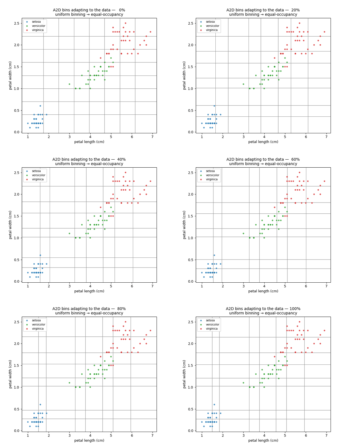
Adaptive or fixed, each feature still encodes to one active bin, one synapse switched on in its space. An A2D over the four features produces a four-entry AAT either way. Adaptation moves only the bin edges, not which spaces exist or how many channels they hold. If you already know the distribution, you can compute the bin edges directly and skip the adaptation altogether.

Adding a bias#

Whether the lanes need a bias at all depends on the encoding. Back in Chapter 5 a bias-free node could only draw boundaries through the origin. That is why the overlapping two-synapse encoding there could not reach every state. The same chapter showed the way out: spread the inputs into a balanced encoding, every pattern lighting the same number of channels. The A2D gives exactly that, one active bin per space, so the encoding itself supplies the freedom a bias would. A separate bias is often unnecessary here. When you do want one, it is just always-on inputs. The ConstantEncoder ignores the value, always lights the same channel, and does not adapt. Stack it onto the A2D with compose, which lays their AATs end to end:

from ktram_neural_core.encode import A2DEncoder, ConstantEncoder, compose

encoder = compose(
    A2DEncoder(dims=4, bits=3, init_min=X_tr.min(0), init_max=X_tr.max(0), l=0.01),
    ConstantEncoder(),                 # one always-on synapse — the bias
)
# encode([5.1, 3.5, 1.4, 0.2]) -> (b0, b1, b2, b3, 0);   space_sizes [8, 8, 8, 8, 1]

That gives five spaces: four adaptive bins, then the always-on bias channel. The Iris example keeps the bias even though the balanced encoding does not need it. One extra always-on synapse costs little and shows the mechanism. init_min/init_max seed each feature’s starting grid from the training range. Features on different scales, sepal length against petal width, each get their own bins with no separate normalization step. The composed AAT is the only thing the lanes ever see, and we hand it to the classifier for the rest of the chapter.

Adapt, then freeze#

Adaptive bins move while they settle, and a moving encoding forces the lane to chase a target that slides out from under it every example. It’s usually best to lock the encoding to keep the representation stable Not always. Real data drifts: a sensor ages, a customer’s habits change, a season turns. An encoder frozen on last year’s distribution ends up spending its resolution in the wrong places, and no amount of lane training fixes an encoding that no longer matches the data. The way out is not a choice between adapting and freezing but a separation of timescales. Leave the bins migrating with the rate l set low enough that the encoding holds still over the span the lane needs to learn, and the slow drift gets tracked instead of chased. The lanes never stop learning either, so they follow the encoding as it shifts underneath them. Iris is a fixed table that will never drift, so here we simply freeze. . So the training runs in two phases, in order.

First, with the classifier switched off, walk the training data through the encoder and let the bins migrate until they settle. Then freeze the encoder and train the lanes against that fixed encoding. The gif above is the first phase. Once it stops, the grid holds still, and every flower lands in the same bins every time.

clf.fit(X_tr, y_tr, epochs=5, encoder_epochs=5)

encoder_epochs=5 is phase one — five passes adapting the bins, then freeze. epochs=5 is phase two — five supervised passes over the frozen encoding. One call runs both, in that order.

Supervised Learning#

Every chapter until now drove the lane with RU, the simplest unsupervised instruction. Paired with the FF read, it gave us unsupervised AHaH plasticity and attractor states that turned out to be logic functions. Supervised learning is more traditional, and in many cases more useful.

Take one labelled flower, AAT encode it, and activate all three lanes. Read each lane with a full-voltage FF to get the lane’s activation. Then provide conditional feedback depending on the label:

aat = encoder.encode(flower)
for lane in range(3):                    # three labels, three lanes
    y = core.evaluate(aat, "FF", lane)
    if lane == correct_label:
        core.evaluate(aat, "RH", lane)   # this IS the class — drive the answer up
    elif y > 0:
        core.evaluate(aat, "RL", lane)   # wrong lane caught saying yes — drive it down
    else:
        core.evaluate(aat, "RF", lane)   # wrong lane correctly saying no — leave it be

Three cases, and they are the whole supervised rule. The lane that owns this flower’s species gets RH, driven up toward yes — these inputs should make it fire. A lane that does not own the flower but said yes anyway is a false positive, so it gets RL and is driven down toward no Not always. As we will see later in this chapter, punishing the false positive maximizes the classification margin, which is exactly what you want when the answer is a verdict. But when you intend to sample the weights stochastically rather than read a winner off them, it is usually best to drop this case. We call the rule with the punishment hard and the rule without it soft. . A lane that does not own the flower and stayed below zero is already right. It gets RF, a plain reverse read that undoes part of the anti-Hebbian FF — the kT-RAM equivalent of “all good bro”.

This is essentially a perceptron written in kT-RAM instructions. Punish the lane when it is wrong, reinforce it when it is right, one example at a time. There is no batch and no stored gradient. The same rule wears a lot of names depending on who is telling the story. The neural-net literature calls it the delta rule or the Widrow-Hoff least-mean-squares update, and anyone coming from optimization calls it online or stochastic gradient descent. A neuroscientist would call it an error-driven Hebbian update — fire-together-wire-together, gated by whether the answer was right. They are all the same move: read the output, compare it to the label, and shift the weights a notch in the direction that would have helped.

The winner is the prediction#

Training drives the synapses with full-voltage reads, because you want those reads to move the weights. In this particular routine, we are either rewarding with RH, punishing with RL, or ‘regularizing’ with FF-RF Regularization is anything that stops a model from fitting its training data too tightly. It usually works by pulling weights back toward neutral, so the model generalizes to examples it has not seen instead of memorizing the ones it has. The textbook version is weight decay: shrink every weight a little on each update. Here it falls out of the instructions themselves. FF is anti-Hebbian and pulls the lane’s output toward zero, and RF only undoes part of that, so a lane that was already right relaxes slightly toward the middle instead of hardening. . Inference is the opposite — you want the prediction without disturbing what you learned. So read each lane with FFLV, the sub-threshold read that reports the weight without changing it. Collect the three outputs and take the winner:

from ktram_neural_core.recode import Winner

scores = [core.evaluate(aat, "FFLV", lane) for lane in range(3)]
prediction = Winner().recode(scores)    # (argmax,) — the loudest lane wins

Winner is just argmax — the lane with the highest output is the predicted class. Reading three lanes and taking the most active is a collective operation. It happens across lanes, not inside one. Putting it together, the entire classifier is short:

from ktram_neural_core.classify import LinearClassifier

clf = LinearClassifier(encoder, labels=[0, 1, 2], model="byte", init="low", seed=0)
clf.fit(X_tr, y_tr, epochs=5, encoder_epochs=5)     # adapt + freeze, then train
pred = clf.predict(some_flower)                      # encode -> read lanes -> argmax

model="byte" puts an “8-bit memristor” at every synapse, so this is the lane running on a device with real quantization. Swap this out for model="mss" or the other model types to see how it works with different levels of device realism.

Technical abstraction layers#

Everything we have done thus far has driven kT-RAM instructions by hand. One instruction at a time, one lane. Read the analog y and branch on it: FF, look at the sign, then apply RH/RL/RF depending on the labels. Or use FFLV for non-adapting inference and take the winner. Let’s call this low level L0 — the bare kT-RAM instruction set, one instruction on one lane at a time. It is how you find out what the parts do. Reach for it in a single-synapse lesson, or any experiment where you want to watch every read.

But we will run this supervised classifier routine constantly from here on. It reads a whole group of lanes first, then acts on what they say. To teach, it uses the labels to drive the right lane up and the confident-wrong ones down. To classify, it just takes the winner. It also cheats. The Python reaches into the emulator and reads each lane’s analog output Vy as a floating point number. Hardware could do the same — put an analog-to-digital converter on every lane — but an ADC per neuron is exactly the bad idea I have already harped on at length. If lane outputs are going to feed anything downstream, they need to come back as AATs, not floats.

We call the hardware that turns a group of analog lane voltages back into AATs an “AAT Recoder”. That covers the reading half of our classifier. The teaching half applies kT-RAM instructions conditionally, branching on the read voltage and the supervised labels. Wrap both halves behind a clean digital interface and you have a second technical abstraction layer, L1. L1 structures are what we will actually build in commercial hardware, where it’s not a matter of exploring the instruction set but rather doing real work. Our first one is RankCut. The name describes its readout — rank the lane outputs, cut the list to the most active. That readout plus the three-case feedback is what makes this particular recoder a classifier. It comes as one object with two calls, adapt to teach and read to answer:

from ktram_neural_core.aat_recoder import RankCut

rec = RankCut(core, labels=[0, 1, 2])
rec.adapt(aat, {label})   # teach: FF read on each lane, then RH/RL/RF by label
rec.read(aat)             # answer: FFLV read on each lane, recoded to an output AAT

Underneath, those two calls are the exact instructions we wrote by hand a moment ago — same FF, same three-way feedback, same low-voltage read.

In full, the readout returns the addresses of the lanes above a threshold — zero volts, say — strongest first, and cuts the list after at most N entries.

The rank-cut in hardware#

Taking the single winner is the easy readout. Often you want more — the top two or three in order, or every lane that came out positive, ranked. Those are all one operation: sort the lanes by output, drop the ones below a threshold, and stop after at most N. That is the rank-cut, and the winner is just its smallest setting — threshold at the floor, N of one.

Sorting analog values the obvious way means an analog-to-digital converter on every lane and a digital sort algorithm behind them, which would take a pile of silicon. There is a much cheaper trick, and it is the kind that makes hardware fun (at least for me!).

Every lane hands you a voltage — its output Vy, sitting somewhere between −V and +V. Take one reference voltage, shared by all the lanes, start it above the top of the range, and sweep it down. Each lane has a comparator watching its own voltage against that falling reference. The instant the reference drops past a lane’s voltage, that lane’s comparator trips and the lane calls out its address.

Picture a flood draining off a landscape. As the waterline falls, the highest peak breaks the surface first, then the next, then the next — and if you write down the order they appear, you have sorted them tallest-first without measuring a single height. The swept reference is the waterline and the lanes are the peaks. The strongest lane trips first, the next strongest second, and the addresses come out already in rank order. Stop the sweep when the reference reaches the threshold — everything still underwater is a no — or after N lanes have surfaced.

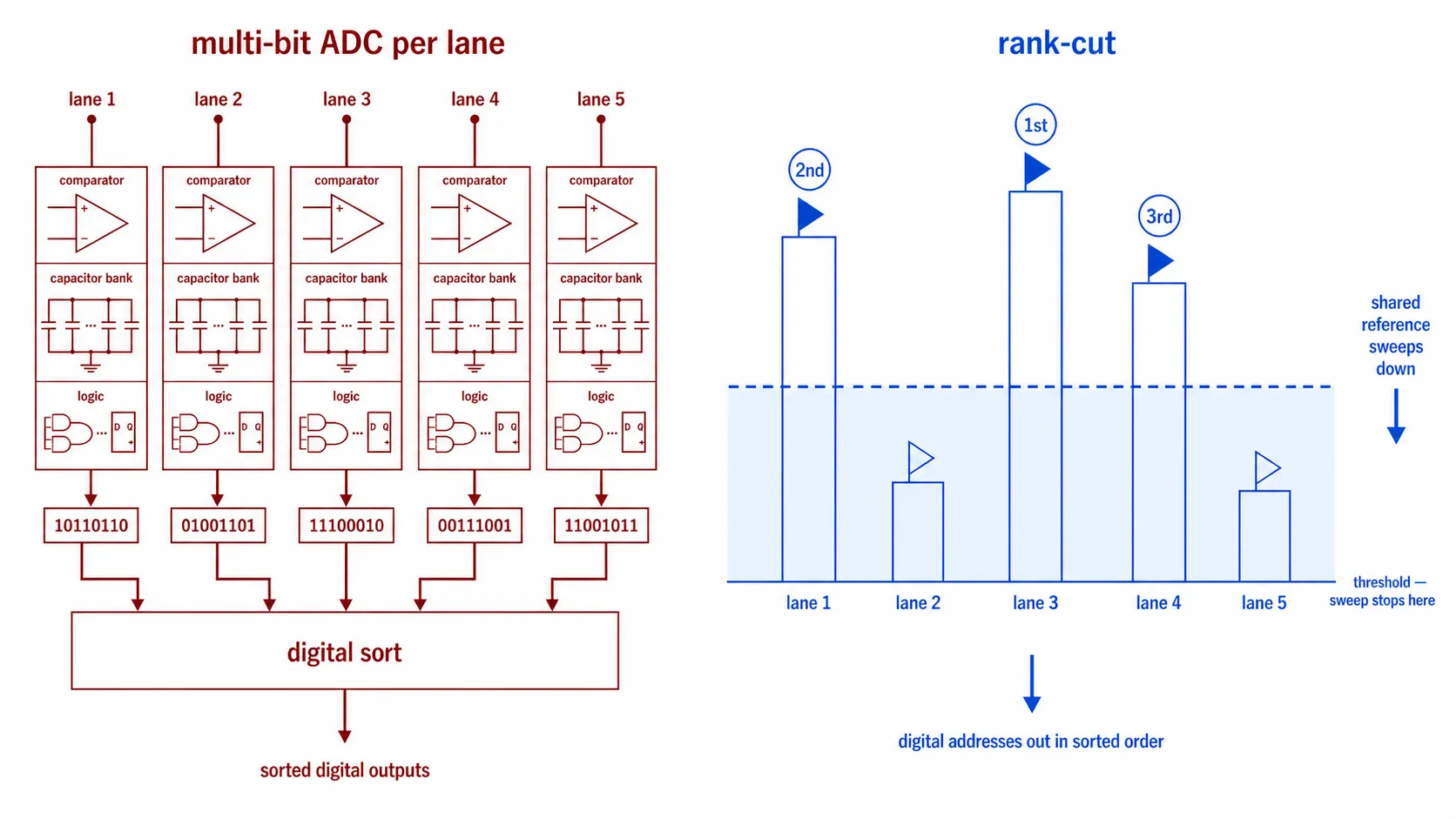
Look at what that saves. The ADC route puts a full converter on every lane: a comparator, a capacitor array, and conversion logic. Then it ships all those digitized numbers off to a sort engine with the memory to hold them. That shipping is the expensive part: most of the energy in CMOS goes into charging and discharging the wires that carry bits between blocks, not into the logic itself. The swept reference keeps everything local — one ramp shared across the array, one bare comparator per lane, and a latch to record the order. The sort is done by the time the ramp finishes. It is encoded in when each lane trips, not in a number you had to compute and move. And the answer is the firing order, so you can stop the ramp the moment you have your N or hit the threshold. An easy decision settles early. One sweep of time saves a lot of silicon and a lot of energy — exactly the trade you want on hardware meant to save energy.

Does it work?#

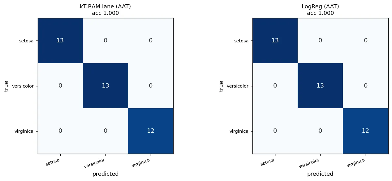
Accuracy on its own says little. What matters is how the lane compares to a real linear classifier given the exact same inputs. The AAT encoder is doing some work and a fair test has to hold it fixed. So I freeze the A2D encoder once and run three things on the identical AAT encoding: our kT-RAM lane, scikit-learn’s LogisticRegression, and a LinearSVC. All three are linear classifiers. The reference two solve for their weights in one batch over the whole dataset. The lane learns online, one example at a time, with local instructions. A fourth bar, plain logistic regression on the raw measurements, shows what the encoding itself costs or gains us. The question is whether the new L1 RankCut routine lands where the batch solvers do.

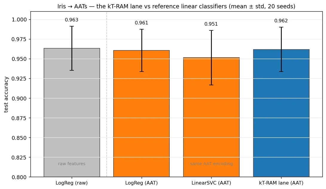
Each lane sees only its own weights and its own read. That online rule still lands on the same accuracy as a batch solver holding the entire dataset in memory.

Where the misses land#

The twenty-seed average was 0.962, not 1.0, so on some splits the lane misses a flower or two. Which flowers, and why? Iris has four measurements and the lane reads all four at once. Any 2D plot is just one shadow of that four-dimensional data, so here are three of them:

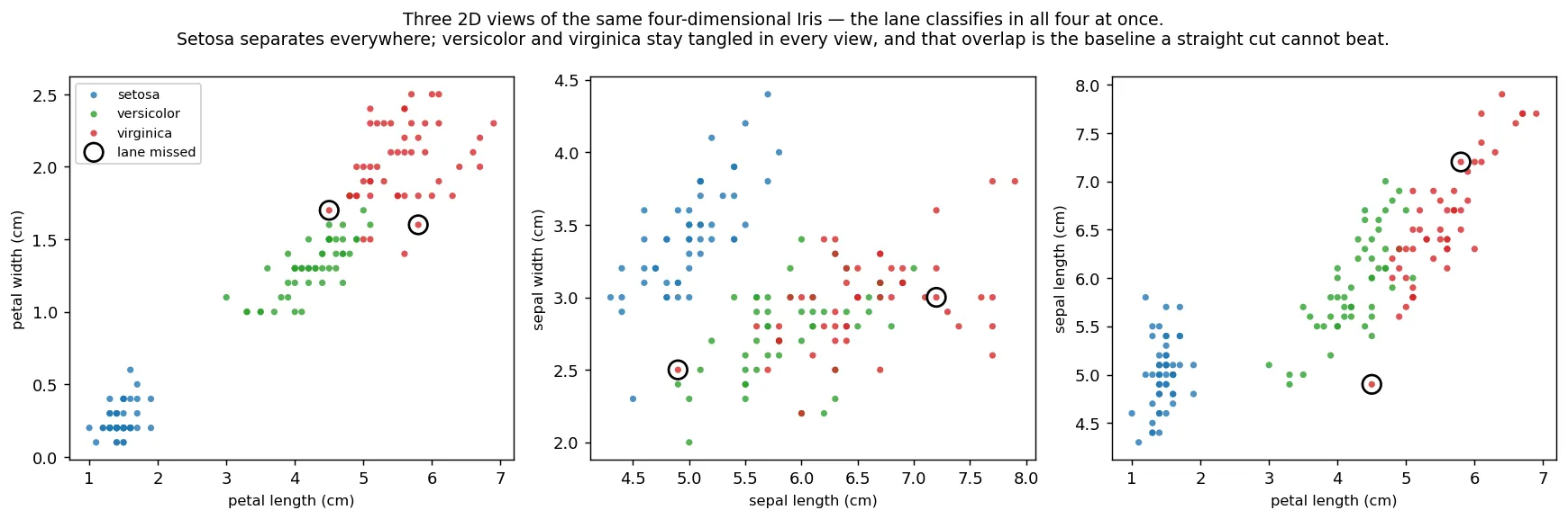
The lane and logistic regression miss the same flowers, the ones in the versicolor–virginica overlap. Those are the support vectors from Chapter 5b that no single line can satisfy at once. That is a property of the data, not the learning rule.

So the ceiling is expected, and hitting it is the point. One cut per class, learned with local instructions, lands exactly where the standard linear solvers do. Getting past that straight line takes more than one cut. (we will get there soon)

Reading at temperature#

Inference read each lane with FFLV — quiet enough that the winner comes out the same on every read. Every kT-RAM read carries the kT-bit’s read noise, and we have two dials for it Both dials come straight out of Johnson–Nyquist noise. Any resistance at temperature $T$ carries a random voltage across it, thrown off by the thermal motion of its own carriers, of size $v_n = \sqrt{4 k_B T R \Delta f}$. Here $k_B$ is Boltzmann’s constant, $R$ is the resistance the junction node sees, and $\Delta f$ is the bandwidth the read integrates over. Nothing in that expression depends on the read voltage, so the hiss is a fixed number of volts while the signal you are reading scales with $V$. Referred to the weight, the ratio grows as $1/V$: dial one. The read pulse sets the bandwidth, $\Delta f \approx 1/2t$, so a longer pulse averages more of the hiss away: dial two. : the read voltage and the read pulse width. The thermal part of the hiss grows as $1/V$, and it grows again as the pulse gets shorter, because a longer read integrates the hiss down. We turn the voltage here, with a noise fraction that scales it down by $1-\text{noise}$. At the standard low-voltage read the result is nearly clean. As $V$ drops toward zero the hiss swallows the signal.

y = core.evaluate(aat, "FFLV", lane, noise=0.6)   # read at (1 - 0.6) x 0.05 V = 0.02 V

Turn that dial and the winner is no longer settled in advance. Each lane reports its true voltage plus a random kick, and the argmax becomes a draw. It is weighted toward the loudest lane, but a close runner-up with more noise can take the win. For a setosa nothing changes. Lane 0 is so far ahead that no plausible kick unseats it. For a flower on the versicolor/virginica overlap, the two lanes read within a whisker of each other, and the hot read returns versicolor on some reads and virginica on others. The classifier stops issuing verdicts and starts drawing samples.

Whether those samples mean anything depends on what the weights hold, and one line of the training routine decides that.

Soft and hard feedback#

Go back to the three-case rule and look at the middle case: a wrong lane that fired anyway gets RL, driven down. That one line decides what the lanes become.

for lane in range(3):
    y = core.evaluate(aat, "FF", lane)
    if lane == correct_label:
        core.evaluate(aat, "RH", lane)
    elif y > 0:
        core.evaluate(aat, "RL", lane)
    else:
        core.evaluate(aat, "RF", lane)

for lane in range(3):
    y = core.evaluate(aat, "FF", lane)
    if lane == correct_label:
        core.evaluate(aat, "RH", lane)


    else:
        core.evaluate(aat, "RF", lane)

Keep it and the feedback is hard. A lane is punished every time it speaks out of turn, so the stable outcome is one loud lane per region of input space and every other lane pushed below zero. Hard feedback carves the decision boundary, maximizing the decision margin.

Drop it and the feedback is soft. The wrong-but-fired lane falls through to the RF case with everyone else, so no lane is ever driven down for firing. A lane climbs when its label is the right answer and holds its ground otherwise. Where the classes genuinely overlap, both lanes stay above the threshold instead of one being beaten under. Hard feedback keeps the single best answer and silences the rest. Soft feedback keeps every answer the data supports in the running. In the emulator this is one argument: rec.adapt(aat, {label}, feedback="soft").

Hard weights and a cold read are the typical classifier’s domain, where we want to maximize the decision boundary and punish indecision. Soft weights and a hot read are a different machine: shown a flower from the overlap, it answers versicolor on some reads and virginica on the rest, because the training data never settled the question either. The important part here is that the noise is conditioned by the weights, which means our samples will produce more variance around the areas of uncertainty.

Label in, pattern out#

A group of kT-RAM neural lanes runs one direction: an AAT goes in, and an AAT comes out. Nothing says which side the labels sit on. The classifier learned the pattern-to-label mapping. You cannot hand those trained lanes a label and get a flower back — the mapping is the wrong direction. A generator is a new set of lanes that learns the opposite mapping. They are trained separately, on the same data, with the same basic supervised routine. The label enters as a plain input coordinate, and the output channels stand for pattern bins.

Take a flat two-dimensional dataset — points on a plane, each carrying a class label. Bin both axes with the fixed-bin A2D from earlier, five bits per axis for thirty-two bins each. The widget below has a resolution knob, so you can sweep this. To classify we did the obvious thing: one lane per label, reading the bins. To generate, swap the roles. Thirty-two x lanes, one per x bin, read only the label. Thirty-two y lanes, one per y bin, read the label together with the x bin. Together those sixty-four lanes are the generator. Teach them soft. Teach them with slightly hot reads, too. The hiss dithers the byte-quantized updates, smearing hard rounding thresholds into smooth averages. Audio engineers have used the same dither trick for decades. Here the physics does it.

The classifier’s lanes start at the low init, every conductance near its floor. The generator lanes start at the medium init, every conductance near mid-scale. A lane’s hiss scales as one over the square root of the total conductance the read sees, so the smallest-magnitude lane is the loudest. Start the generator lanes at the floor and every untrained lane out-shouts the trained ones on every hot read, and the samples are noise. The mid-scale start loads every lane with “magnitude ballast”. An untrained lane reads near zero and stays quiet until training moves it.

To draw one sample, clamp a label and read the x lanes hot. The most active lane is an x bin — commit it. Then read the y lanes hot, given the label and that committed x, and the winner is a y bin. Decode the two bins back into a point, and that is the entire generator.

The sequence is critical, so slow down and pay attention. The number of steps is not a design choice. It equals the number of tuples in the AAT we are generating. This dataset is two-dimensional, so the output AAT has two tuples, an x symbol and a y symbol, and one sample takes two reads. An AAT with $k$ tuples takes $k$ reads. The rule at every step is the same: read the lanes for one tuple given the label and every symbol committed so far, take the most active, commit it, move to the next tuple. That is the chain rule of probability, $p(x, y) = p(x)\,p(y \mid x)$, running as lane reads. From here on we call the whole sequence of reads the chain.

The split into x lanes and y lanes is how the chain is organized, not a hardware requirement. A lane simply ignores any input space held at NONE, so you can pool everything into one array of lanes whose input spaces cover the label, the x bin, and the y bin, with one lane per symbol across all three — sixty-seven lanes here. The chain runs the same way. Clamp what you know, hold the rest at NONE, read the lanes of one unknown space, commit the most active into that space, and move on to the next. That is an auto-associative array: clamp any subset of the entries and the chain fills in the rest. Clamp the label and it draws a pattern. The generator in the widget is this array with its rows split apart, which keeps the display legible.

What the sequence captures is the agreement between the tuples. Lanes that see only the label can report one thing: how often each of their bins gets used by that class. That is a marginal. They have no way to report that y runs high whenever x runs high, because nothing in their input says which x we are on. Committing x changes the question the y lanes are asked. Instead of “where does this class put its y mass,” it answers “where does this class put its y mass on the slice of the plane at this particular x.” If the class is a tilted cloud, those two questions have different answers, and only the second one draws the tilt. Skip the commit and read the x and y lanes at the same instant, each side seeing only the label, and every draw comes from the two marginals instead. The histograms still match, but the tilt flattens into an axis-aligned blur, because nothing ties any particular y to the x it came with. The widget below has a switch for exactly this, chained against synchronous, so you can watch the correlation appear and vanish. Run the same chain over hundreds of tuples instead of two and you have the image generator a few chapters from now, each read filling in one more piece of the picture while looking at every piece already filled in.

So here it is. Press Start, and lanes train and generate 2D Gaussian clusters live in your browser. The left panel holds the data and the classifier. You can add, drag, tilt, and relabel the Gaussian clouds, and three label lanes trained hard underneath color every cell of the plane by its cold winner. Drag a cloud across the plane and the boundary chases it, because the lanes never stop learning. The right panel is the generator: the soft x and y lanes drawing samples at whatever temperature you set, with marginal histograms along the top and side comparing what it draws against what the data holds.

Try a few things. Drag the temperature to zero and the samples collapse to one spot per class — with no hiss the chain can only ever pick its single loudest bin pair. Raise it and the cloud fills back out. Push it far and the samples start spilling past the data. In between, the histograms settle onto the grey reference curves, and warmer reads trace the shape better than cool ones, because the noise is doing the mixing. Load the tilted preset and the generated cloud comes out visibly tilted, the chain carrying the correlation. Now flip the draw from chained to synchronous. The x and y lanes read at the same instant, each side seeing only the label, and the tilt collapses into an axis-aligned blur while the marginal histograms barely move. The joint structure was never held in the x lanes or the y lanes alone. It rode on the committed x passing from one read to the next.

Then flip the feedback to hard and watch what the punishment does. The RL case starts beating down every lane that fires out of turn. In a generator that is nearly every lane on nearly every example, because the answer is genuinely spread across many bins. The read always returns its most active lane, so the samples keep coming, but within seconds they stop looking like the data. A generator punished for every wrong guess cannot hold a spread. It can only hold a single best answer, and everything else gets beaten flat. Flip back to soft and the distribution fills back out.

Where we are#

We used three lanes over an A2D encoding, one lane per label, trained with a simple kT-RAM instruction set routine. Read cold, that lane matches batch logistic regression and a linear SVM. Read hot, and the same routine keeps the odds instead of the verdict. Teach fresh lanes the opposite mapping, chain the reads, and they draw patterns instead of naming them.

Count what two memristors wired against each other and a handful of voltage patterns have done so far. They held a bit against the thermal bath in Chapter 3, were memory or logic or inference by choice of partition in Chapter 4, assembled logic gates from the structure of the data in Chapter 5, and found the maximum-margin boundary in Chapter 5b. Here they land on logistic regression, then sample a joint distribution when softened, read hot and sequenced. We added no new devices or circuits or instructions, and we have barely started.

Next: Chapter 6b: The Basis Encoder