Chapter 4: The Neural Lane

There are so many things that can be built with kT-bits that it’s almost paralyzing to pick just one. But this series needs to focus, and I’ve already picked one—something I call a neural lane. A neural lane is actually a sub-type of ‘kT-RAM’, a substrate where we can pick one or more kT-bits and drive kT-RAM instructions. Let’s start with that.

What kT-RAM actually is#

kT-RAM — Thermodynamic RAM — is a construct: an abstraction that sits above the specific implementations. Take a pile of synapses (the kT-bits from Chapter 3, each a differential pair of memristors), make any subset of them individually addressable, and give yourself a set of voltage drive patterns — instructions — that select bits, sum their currents, and adapt their conductances in one motion. That’s the basic idea. Reading the memory is computing with it. No fetch, no separate ALU, no trip out to DRAM and back. Memory access is synaptic access is compute.

Three things fall out of that definition:

• It says nothing about layout. kT-RAM is addressable synapses plus an instruction set. How you physically arrange them — the topology — is left wide open. A binary tree, one fat neuron, a crossbar: all are kT-RAM if you can select kT-bits and drive them. It goes without saying, but if you match the topology of the kT-RAM implementation with the topology of the networks you are interested in, you will reap benefits in efficiency.
• It says nothing about the substrate. You can emulate kT-RAM in software at whatever precision you want — we keep a family of interchangeable cores for exactly that — or build it in CMOS, or in memristors. Same instructions, same routines, swappable underneath. That’s how we write and test the algorithms now and drop in real devices later without tearing up the stack.
• It’s one fabric for memory, logic, and learning. The same selected-and-driven synapses are RAM when you read them, a logic gate when you couple a few of them, and a classifier when you couple even more.

So kT-RAM is the genus. What we define in this chapter, the neural lane, is a species.

Don’t Bite Off More Than You Can Chua#

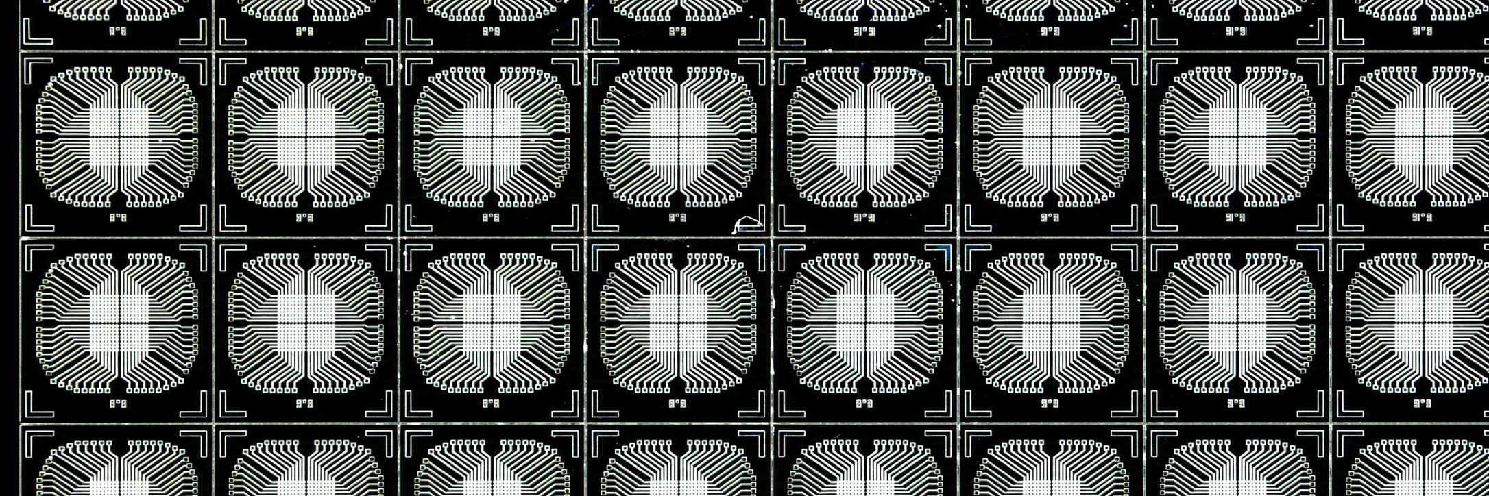
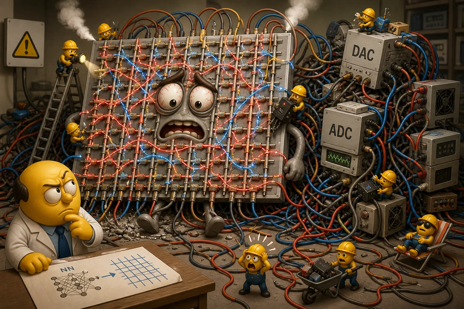
The typical way to approach memristor crossbars is to utilize their natural topology. Lay the devices out in a grid, store a weight as the conductance at each crosspoint, drive voltages down the rows, and read the currents off the columns. Out pops a vector-matrix multiply in a single shot. On paper it is glorious. We already watched it fall apart in the lab back in Chapter 1 — sneak paths, hungry DACs and ADCs, device variation, topology mismatch.

The job we keep handing them is the trap. So let’s hand it a different job.

The unit crossbar concept is simply to use one memristor at a time from a crossbar at any given time. If you keep the arrays small enough, 32×32 or less in size, it’s possible to read and write individual devices without the sneak path currents totally ruining your day. Of course, one memristor does not a neural network make. If only one memristor at a time is going to be accessed, we will need to have a bunch of them that we can couple together in some way—and that’s roughly how we will be building ASSIMILAATE Neural Lanes. From a sea of crossbars—not just one.

The unit crossbar#

Take a crossbar and shrink it until the sneak paths can’t hurt you (A), then wrap it so that, from the outside, it behaves like a single addressable memristor (B). That’s the unit crossbar. We are going to completely ignore its topology and treat it as simply a carrier of individually selectable memristors.

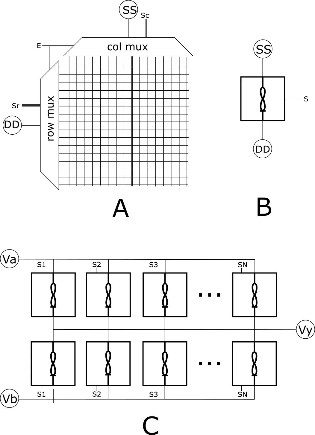
Panel A is a 16×16 array. The size is arbitrary and in general “the bigger the better” so long as sneak paths and other non-ideal effects don’t fully take control. A row multiplexer and a column multiplexer hang off the edges. Feed the row mux an address on Sr and the column mux an address on Sc, and where the chosen row crosses the chosen column, one memristor gets coupled between two lines: a source line SS and a drain line DD. Every other device sits idle. You can drive the non-selected columns and rows to zero (more complicated, less cross-talk), or leave them floating (less complex, more cross-talk). The enable line E switches the whole array on or off, so a unit crossbar can also be told to select nothing at all—an open circuit. In our build we will simply leave the non-selected rows and columns floating. This can and does lead to sneak paths, but we have a plan for that. Indeed, by the time we are done, hopefully the annoying crap that memristors and crossbars dish out—the stochastic switching, the sneak paths, the slight variability between devices—will all get ironed out. Not by fighting it, but rather by changing our understanding of what the ‘architectural building block’ of neural computation actually is.

One device at a time, between two lines. At 16×16 the sneak paths are small enough that you can read and write that one device relatively cleanly — no selector transistor at every junction. The address that names a device is log₂(Nr) + log₂(Nc) bits: for a 16×16 array, four bits of row plus four bits of column, eight bits to pick any one of 256 memristors. Bigger is definitely better here, so if your memristor crossbars have selector devices or act as diodes, etc., then you can go much larger, and that’s a good thing. My point is not that you need small crossbars—it’s that if you don’t have anything else it’s not the end of the game. We can still build something useful—which is good because I have hundreds of small crossbars sitting in my clean lab.

Panel B is my symbol for a unit crossbar. S carries the row bits, the column bits, and the enable bit folded together, i.e. the selection bits. Select an address and it couples the corresponding device to the input and output lines (SS/DD). Turn it off and it’s an open circuit. Give it an address, get one device back — or none. Couple dozens or hundreds or thousands of unit crossbars together and the parallelism comes back at the next level up. It’s also clear now that a ‘crossbar’ is not even necessary. One could dream up other arrangements of individually-selectable memristors in ‘another embodiment’, as patent lawyers like to say.

Wiring a neural lane#

In Chapter 3 the kT-bit was a differential pair of memristors, and its weight is the difference between the two conductances — a signed number that can push a neuron toward firing or pull it away. In other words, a signed synapse. All we do here is build each half of that kT-bit from a unit crossbar and stack the two halves in series between two voltage rails. The a-side device sits between the top rail Va and the output node; the b-side device sits between the output node and the bottom rail Vb. The pair is a voltage divider — the same 2-1 series circuit worked out device-by-device in Chapter 3b — and the node between them settles wherever the more conductive side pulls it. Make the a-side more conductive and the node climbs toward Va (positive); make the b-side more conductive and it drops toward Vb (negative). Same kT-bit you already built on real devices, now reached through two unit crossbars.

Panel C lines up three synapses — S1, S2, S3 — between the same two rails, Va and Vb, and ties every pair’s midpoint to one shared output line, Vy. Drive the rails, and the selected synapses act as voltage dividers wired in parallel onto Vy. By Kirchhoff, that node settles to the activity-weighted average of the selected weights:

$$y = \frac{\sum_{i \in \mathcal{A}}\left(G_{a,i} - G_{b,i}\right)}{\sum_{i \in \mathcal{A}}\left(G_{a,i} + G_{b,i}\right)}$$

where $\mathcal{A}$ is the set of synapses you selected. The output is one analog number, and because it’s a ratio it stays in [−1, 1] no matter how many synapses you switch on — two for a logic gate or thousands for a classifier.

Which synapses get switched on is decided by an Activation Address Tuple, or AAT — an ordered list of integers, one per address space:

$$z = (a_0, a_1, a_2)$$

The first integer picks a synapse in S1, the second picks one in S2, the third in S3, and so on. Position matters: the same number means a different device depending on which slot it sits in. Each address space can be a different size, so we sometimes write a single selection as [6/64] — channel 6 out of 64 — and a full tuple as

$$z = [\,6/64,\; 2/32,\; 45/64\,]$$

The tuple is sparse. Out of every device on the lane, exactly three (in this case) are doing anything on a given evaluation: one per space, set by the three integers.

The AAT does no translation. The tuple is the wiring pattern: the order of the addresses and the sizes of the spaces are the physical layout of the lane, pin for pin. Nothing sits between the integers and the devices — no routing table to consult, no address map to maintain. Broadcast the same AAT to a hundred different lanes and each one reads it against its own local synapses. The constraint that the tuple must be ordered and split across fixed-size spaces looks like a limitation until you notice it has quietly deleted the entire hardware-mapping problem.

Of course we now have a new problem called “AATs”. This looks like a binary vector, but it’s not exactly. It certainly does not look like what most modern neural networks utilize. It’s a seemingly special or niche encoding. Your first reaction is probably skepticism and perhaps, if you are weak of mind—to walk away. That would be a mistake, because it’s entirely possible to convert datastreams of many flavors into AAT streams, often trivially, and in some cases the data was really an AAT stream but nobody noticed. An RGB pixel is already an AAT: three numbers, each an address into a 256-channel space — [R/256, G/256, B/256]. A line of ASCII text is a stream of single-address AATs into a 256-symbol/channel space. Digital integers are also written as an AAT stream. Take the number 42, for example. That could be 42/50, or it could be [4/10,2/10], or other AAT representations. Most digital encodings are the same story once you look: an index into a fixed set of choices. Nobody calls them AATs, but that’s what they are. Our digital world is already built with AATs.

Continuous communicated values are the fantasy#

We talk about neural networks as if they run on real-valued, floating-point numbers, and as a piece of physics that is a little ridiculous. A floating-point number is already digital: a finite pattern of bits, one rung on a discrete ladder of values we agree to read as a stand-in for a real number. The continuum is an interpretation we paint over those bits. It was never in the silicon, and it was never on a neural wire either.

There is a hard-won reason for that. Communicating analog values is only viable locally; push an analog signal down a long wire and noise, attenuation, and crosstalk eat it alive. Digital computing learned this lesson early and decisively, which is why we quantize, send digits, and rebuild the smooth quantities we want once we arrive. Biology made the same call: a neuron communicates in discrete spikes, not a continuous voltage broadcast across the brain. The native language of a physical neural network, grown or fabricated, is digital. The idea of communicating continuous values in a neural network is a fantasy of the human mind.

An AAT is the encoding that agrees with both lived engineering experience and biology. The genuinely strange thing is the status quo: we run real-valued neural networks on digital computers, spending enormous effort to simulate a continuous communication scheme that no physical substrate would actually use. We built a digital machine because analog did not work, taught it to pretend it is analog, and then try to map continuous value neural networks to it. Communicating neural state as AATs drops the pretense. Iron out that one wrinkle and everything downstream falls into place.

Another detail that we have not yet covered, but will: y comes out analog, which means this picture isn’t finished. Somewhere downstream that analog activation has to be turned back into AATs, and that recoding step is its own article. For now the thing to hold onto is the structure in Panel C: addresses in, one stacked pair per space between two shared rails, a normalized differential voltage out on Vy. We call that structure a neural lane. We will combine multiple neural lanes together, either in parallel or temporally multiplexed, to form our output AATs. This collective step will be our “A2D” operation—it acts on many neurons at once. The thing that turns an analog vector into AATs we call an “AAT Recoder”, and there are a number of ways to do it. We will explore a few in this series.

One lane, many neurons#

A neuron here is a partition of the lane’s address space — a chunk of addresses you agree to treat as one unit. The only thing that separates one neuron from another is information and time, not the hardware itself.

Take the lane in Panel C with each of its three spaces of 256 channels. That’s 768 synapses sitting on one set of neural drivers. What can you do with them?

• Treat the whole lane as one neuron: a 3-entry AAT reaching across all 768 synapses.
• Cut every space in half — addresses 0–127 (in each space) are one neuron, 128–255 are another — and you have two 384-synapse neurons sharing the neural lane.
• Slice finer and get 128 neurons of six synapses each. Now the neurons are looking more like logic gates.
• Drop to a 1-entry AAT and you’ve recovered a plain addressable bit of memory.

The same lane is memory, logic, or inference depending only on how you carve up the addresses and march the tuples through over time. The hardware never changes. The partition does. That is what divorces the topology of the network from the topology of the crossbar. The thing we have ‘discarded’ is the real-value interpretation of neural activations, and a big part of this project (other than actually fabricating a neural lane with crossbars), is to perform the simulations and open source the code to make it clear that this is a good idea. And to be clear, when I say the goal of this series is to assimilate neural transforms, I mean the modern (but soon to be antiquated) floating-point variety. I’m not asking anybody to change how they train their models—unless they want to, of course.

Memristor to Transistor ratios get better as the crossbars get bigger (but remember the physical constraints). A 512×512 unit crossbar holds 262,144 devices. A lane built from 128 differential pairs of those carries 33.5 million synapses — enough for one enormous neuron, or roughly 670 neurons of 50,000 synapses each, or any split you like, because a neuron is just a memory partition. Decoders, drivers, and sense circuitry can be shared across the core, not bolted onto every neuron.

Time to Code#

We’ve now got the abstraction (kT-RAM), built on the kT-bit, and a topology we will explore first. Next comes some code. We’ll build a kT-RAM emulator around the crossbar neural lane — one that models selecting and driving kT-bits from a unit-crossbar fabric — and start running experiments on it in the next chapter so we can build up some intuition about AHaH attractors before jumping to supervised and unsupervised classification and finally actually building the thing.