Chapter 5b: Maximizing Noise Margin

Chapter 5 drew red lines through the data, counted where they landed, and called the landing spots attractors. We watched a two-kT-bit node fall into one decision boundary or another with no teacher in the loop, and we read those boundaries off as logic gates. What we never said is why. Why does a line settle in one place and not another? Why is that place stable at all, so that a few hundred random nodes drain into a handful of states instead of smearing out across every angle the line could take? That is a question about force — what pushes the boundary, and what holds it once it stops. This chapter is the force.

Do or do not, there is no try#

Start with the failure. In Chapter 5 the output of the node was $y = x_0 w_0 + x_1 w_1$, and the decision boundary was the line where that crosses zero. Pick a boundary at random and you can get something like this:

The line runs right through [1,1]. The node’s output on that pattern is a hair away from zero, which means the node has not decided. Ask it what [1,1] is and it shrugs. Try to write the truth table and you get a column you cannot fill: positive? negative? — the output is so close to the boundary that thermal noise alone could flip it either way on the next read.

You cannot build confident logic from un-confident neurons. A logic gate has to be sure: same input, same answer, every time, even with noise rattling the conductances. So the real job of the learning rule is to drive the node off the fence and hold it there. We need the weights to change in a way that reduces indecision. We need a synaptic plasticity rule.

The rule can only know three things#

Write the weight update as

$$\delta w_j = f(x_j, y, w_j).$$

The update to one synapse is some function of the input $x_j$ on that synapse’s line, the node’s output $y$, and that synapse’s own value $w_j$. It has to be a function of those three things and nothing else, due to locality. A kT-bit is two memristors wired against each other on a lane, and the only quantities physically available to it are its own state, the input driving its line, and the voltage the lane reads out. There is no global error signal piped in from outside, no optimizer holding the whole dataset in memory. Everything that moves the weight has to be local to the weight. That sounds like a restriction, and it is — a useful one. It throws out every rule we could write on paper but never build, and what survives is a short list.

Hebbian explodes, anti-Hebbian decays#

The oldest guess is Hebbian: neurons that fire together wire together.

$$\delta w_j = \alpha\, x_j y.$$

Push the weight in the direction the node already leans. It has a fatal problem. Start a synapse a hair positive, read it, and it reads positive; reinforce it, and it reads more positive; reinforce again, and you are on a positive feedback loop that runs the weight to infinity. Hebbian learning alone is a microphone next to its own speaker.

The fix that suggests itself is the opposite move, anti-Hebbian:

$$\delta w_j = -\beta y.$$

Push the weight against the output. Now the runaway is gone, but you have bought a different kind of useless: the weight decays toward zero and sits there. Anti-Hebbian alone walks every node back to the fence we were trying to escape.

So one rule explodes and the other collapses. Put them in the same rule and they fix each other.

AHaH: Hebbian where you’re unsure, anti-Hebbian where you’re sure#

$$\delta w_j = \alpha\, H(y) - \beta y,$$

where $H(y)$ is the step function — its sign is the sign of the output. This is the unsupervised AHaH rule, the Hebbian and anti-Hebbian halves of the FF-RU cycle from Chapter 5 written as one line. Watch how the balance between the two terms shifts with $y$.

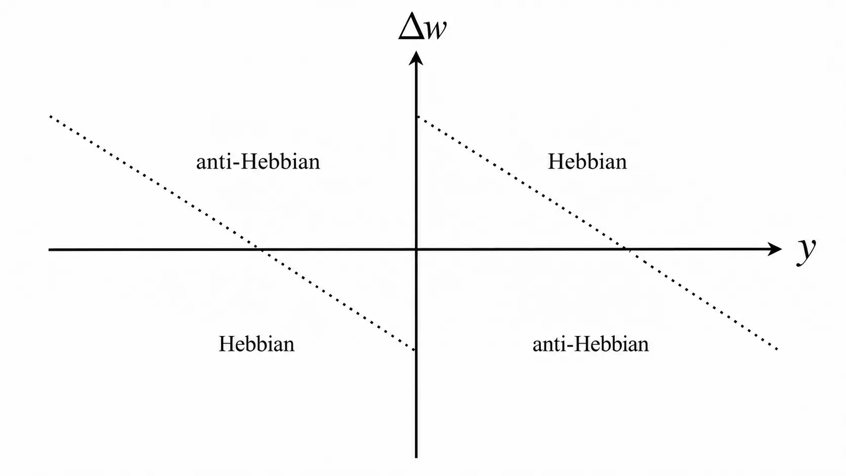
Read it from the middle out. When $y$ is near zero — the node is unsure — the Hebbian term wins and the update is large, so an undecided node gets shoved hard toward a decision. As the node commits and $|y|$ grows, the anti-Hebbian term catches up, the update shrinks, and at some magnitude the two terms cancel and the weight stops. The weight grows fast at first, then slows, then holds at an equilibrium. It is a wedge that drives the node off zero and pins it on one side.

Small activations get large updates, large activations get small ones. The rule spends almost all of its effort on the patterns the node is least sure about, and barely touches the ones it already answers with confidence. In the language of machine-learning classifiers that move has a name — margin maximization. On hardware it has a more physical description: the node is putting distance between its decisions and the noise that could flip them.

The swing-state strategy#

The same idea runs a national election. You are running for president with a fixed pile of money to spend on advertising. Where do you spend it?

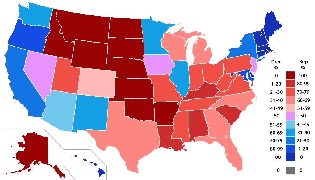
You do not spend a dollar on the states that already vote your way by forty points — those are in the bag, and money there changes nothing. You do not waste it on the states you will lose by forty either. You pour everything into the handful of states that are close, where a push moves the result. The AHaH rule does the same accounting on data. The patterns the node already answers with conviction get almost no update; the close ones, the swing patterns near the boundary, get all of it. A node and a campaign run the same strategy because they face the same problem — a finite budget against a decision that only a few undecided cases will settle.

Reading the boundary as a balance of forces#

Think of the decision boundary as a physical thing that each data point pushes on. When a pattern lands on the wrong side of the line, or too close to it, the AHaH update shoves the line away from that pattern. Each point pushes, and the push is strongest when the line is close.

Pattern [1,1] pushes the line with a force we can call $f_{11}$, [0,1] pushes with $f_{01}$, [1,0] with $f_{10}$. Move the boundary away from [1,1] and $f_{11}$ drops off — but the line has moved toward [0,1], so $f_{01}$ grows and pushes back. Somewhere between them the two forces are equal and opposite, and there the boundary stops. That balance point is the attractor. If you like algebra, write out the weight update for each pattern, sum them, set the sum to zero, and solve — the attractor is the root. If you like pictures, it is the place where the line is wedged between two opposing groups of data, pushed equally from both sides, with nowhere left to drift.

This is why the boundaries in Chapter 5 settled where they did, and why they were stable. A boundary off the balance point feels a net force back toward it. There is an attractor anywhere the data splits cleanly into two groups, because that gap between the groups is exactly where the opposing pushes can cancel.

Those balancing points are the support vectors#

Look at what is doing the pushing when the line comes to rest. The patterns far from the boundary push with almost nothing — they are the locked states, the forty-point landslides. The patterns near the boundary are the ones still pushing hard at equilibrium, and they are the ones holding the line in place. They set where it sits; move one of them and the boundary moves with it, while the distant points could shuffle around freely and change nothing.

A machine-learning engineer has a name for the handful of nearest points that pin a boundary: the support vectors In a support vector machine, the decision boundary is fixed by only the training points closest to it — the support vectors. Points farther away don’t affect where the boundary sits at all. . The empty gap the boundary keeps between itself and those nearest points has a name too — the margin. A line sitting in the middle of the widest gap it can find between the two classes is a maximum-margin classifier, and the points touching the edges of that gap are its support vectors. They are the only data that matters: throw the rest away and the boundary comes out the same. And the fewer of them it takes to hold the line, the more you can trust where it sits — a support vector machine’s error is bounded by the share of the data that ends up as support vectors.

That margin is a noise margin. Digital logic has used the term for decades — the slack between a valid 1 and a valid 0, the buffer that lets a gate shrug off noise on its inputs and still read the right bit. The AHaH margin is the same buffer. The distance from the boundary to the nearest pattern is the smallest output the node ever produces on real data, and that smallest output is exactly what thermal and read noise have to overcome to flip an answer. Widen the margin and every decision moves further from zero. Maximizing the margin maximizes the node’s immunity to its own noise, and on a kT-bit built from two jittering memristors that is a significant detail. It is the problem we opened with — a pattern sitting on the line, one noisy read from flipping. The rule’s solution is to drive every pattern as far from the line as the data allows.

For about fifteen years, from the mid-1990s until deep learning took over around 2012, the support vector machine was the best general-purpose classifier going, and it came with something rare in machine learning — a clean theory of why it works. A model can always draw a boundary that wiggles through every training point exactly, and that is memorization: it has fit the noise, and it generalizes terribly. The widest-margin cut does the opposite. It commits to the simplest split with the most room to spare on either side, and Vapnik’s statistical learning theory showed that the wider the margin, the better the classifier does on data it has never seen — no matter how many dimensions the data has. Maximize the margin and you trade memorization for generalization. That was the seminal result, and it is still the cleanest account we have of the difference between the two.

A wide margin also makes the classifier robust: its answer holds still when you jiggle the inputs, and that robustness is what generalization is. Thermal noise on a read and a never-seen test point are the same kind of jiggle, so the margin that survives $kT$ is the margin that generalizes. Noise immunity and generalization are one claim seen twice.

It doesn’t optimize — it repairs#

A support vector machine solves that global optimization once, over the whole labelled dataset, and returns the single best boundary. Unsupervised AHaH does not. Turned loose from a random start, a node falls into one of many attractors — Chapter 5 counted them and handed them names — and which one it lands in is set by where it began, not by which is best. Every attractor is a clean separation that maximizes its own margin, the boundary wedged in the gap between whichever patterns its basin happened to sort onto opposite sides. The rule maximizes the margin of the boundary it is already near. It never goes looking for the best one, and the support vectors are never computed either — they are just whatever patterns are still pushing when the boundary stops moving.

What it does instead is hold a boundary once one is there, and that turns out to be worth as much. Because every max-margin separation is a physical attractor — an actual low point the dynamics fall toward — a classifier placed on one becomes self-correcting. Train the state however you like, supervised, even with a full support vector machine, to drop it into the exact basin you want. Then hand it to unsupervised AHaH and leave it running. Damage the weights, lose a device, let the conductances drift the way real memristors do, and the same read-then-reinforce loop — local and online, each kT-bit seeing only its own state and the lane’s output — drags the boundary back to the attractor it was sitting in. The damage is a shove off the balance point; the forces that set the balance point shove right back.

This is what vanilla AHaH plasticity does — the bare FF-RU cycle, nothing bolted on. It does not optimize a classifier. It takes a separation between opposing states and makes it stable, turning a maximum-margin boundary — the seminal SVM result, the cleanest line we have between memorization and generalization — into a stable equilibrium of the physics. Place a classifier on that equilibrium and it holds itself there with no teacher and no supervision running, repairing the state as the conductances drift and devices fail.

So far this is one lane, understood from the inside: how FF-RU plasticity moves a boundary, why it settles, and what it settles into. The next step is to put it to work — wire many lanes together, bring in the rest of the kT-RAM instruction set, and build a supervised classifier instead of only stabilizing one. That is where we go next.

When nothing pushes back#

That picture also explains the state we kept hitting in Chapter 5 and could not get rid of — the null state, where the node answers every pattern the same way. It is what happens when there is no opposing force. If every data point sits on one side of the line, every push points the same direction, nothing cancels them, and the boundary just slides until the weights hit the rail. The node ends up declaring everything positive, or everything negative.

Read the null state as the rule reporting a fact about the data: as encoded, it gave the node nothing to separate — no two groups with a gap between them, so no balance point to find. Chapter 5 showed the three ways out, and now they read as three ways to manufacture an opposing force: encode the inputs sparsely so patterns land on both sides, add RA bias synapses that push back against the majority, or be careful with the Hebbian term so the rich do not always get richer. Each one is a way of making sure something pushes the other way.

Where the rule comes from#

None of this is an arbitrary choice of update. You can derive the AHaH rule instead of guessing it. Ask for a node whose output is as bimodal as possible — a clean lump of positive answers and a clean lump of negative ones, with as little mush in the middle as you can manage. That is the no-mumbling condition stated as a statistic, and the statistic that measures it is kurtosis. Minimizing a kurtosis objective over the node’s output is one of the standard routes to independent component analysis Independent Component Analysis — a family of methods that pull a mixed signal apart into statistically independent source components, like separating overlapping voices recorded on one microphone. , the problem of pulling a mixed datastream apart into its independent pieces. Run that derivation and a plasticity rule drops out:

$$\Delta w_i = x_i\left(\alpha y - \beta y^3\right).$$

The exact curve differs from the step-function version, but the two trends are the same: as $|y|$ grows the update first shrinks and then turns anti-Hebbian. Small activations get pushed hard, large ones get left alone. The election strategy and the ICA objective are the same rule seen from two directions — one says spend where it matters, the other says make the output bimodal, and they land on the same curve.

The cores do it on their own#

The real test is whether the hardware obeys this rule, or whether it is a story we tell about it. So run the unsupervised cycle on a batch of emulated cores, record every weight update against the output that caused it, and plot $\delta w$ versus $y$.

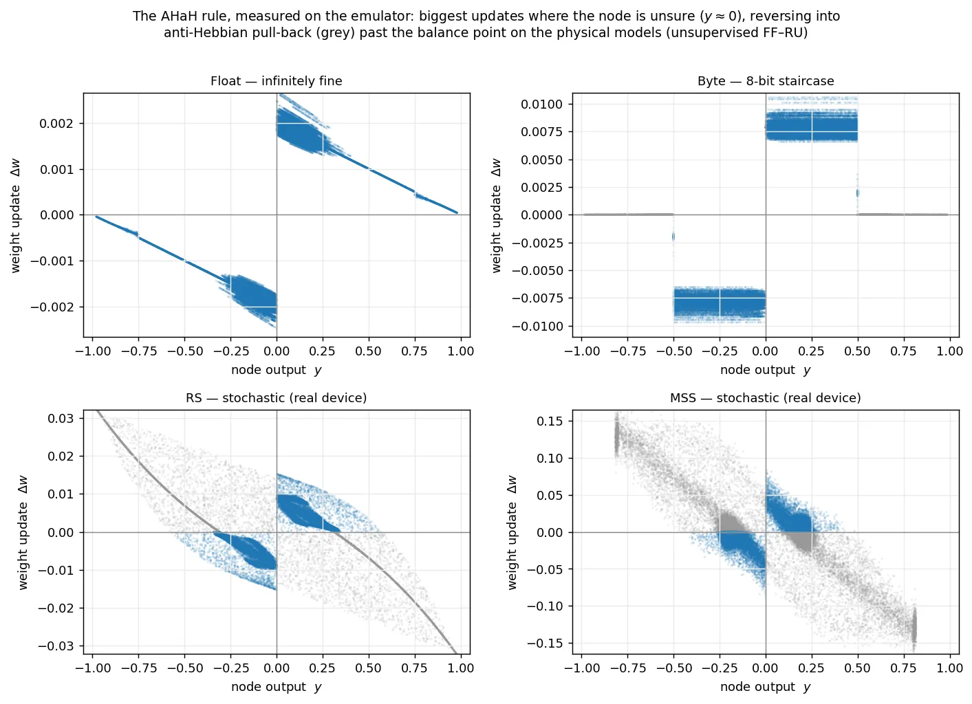
No two cores draw the same curve. The float is smooth, the byte moves in 8-bit steps, and the two physical models, RS and MSS, are stochastic and scattered. The ideal float and byte stay Hebbian and just taper off as the node commits; the physical devices, pushed past their balance point, cross into the anti-Hebbian pull-back that pins the equilibrium — the full wedge from the diagram above, rendered in real device physics. But every one agrees on what matters: the biggest updates land where the node is least sure, near $y = 0$. We did not program the AHaH rule into these cores. We wired two memristors against each other, ran the read-then-reinforce cycle, and the rule is what came out.

A bit against the bath#

Go back to the name. A kT-bit is named for $kT$, the thermal energy of the bath it sits in. That is the jitter that nearly flipped [1,1] in the opening figure. The margin is the wall against it. A state is a bit only while that wall stands above $kT$. Drop it below the noise and the read flips at random — the state is not a bit, it is bath. So the margin is what makes a state a bit at all. Maximize it and you dig the well deep enough to hold a bit against the bath.

Chapter 3b built that wall one bit at a time. A single pair reads clean only when it is polarized and full of evidence. Grow the weight difference and the magnitude, and the signal climbs above the noise floor. Balanced and light, the read is mostly hiss. The AHaH rule does the same thing across a lane, steered by the data. It reads the structure in the inputs, drives each pair off the balance point, and grows the lean that structure calls for. That growing lean is the margin. So margin maximization is barrier-building, run across a whole node. The rule does not fight the noise. It grows the wall the physics already offers.

What we found#

The attractors from Chapter 5 are not arbitrary resting places. Each input pattern pushes the decision boundary away from itself, the push gets stronger as the boundary comes closer, and the boundary settles where the opposing pushes cancel — wedged in the gap between two groups of data, equidistant from the nearest patterns on either side. Those nearest patterns are the support vectors, and each kT-bit settles among them using only what is local to it — no teacher, no global solver. The rule does not search the many possible boundaries for the best one; it maximizes the margin of whichever boundary its basin drops it onto, holds it there as a matter of physics, and repairs it when damage knocks it loose. That margin is a noise margin — the boundary sits as far from the nearest patterns as the data allows, leaving the most room it can between every decision and the noise that would flip it. When the data offers no opposing group, there is nothing to balance against, and the node slides into the null state.

Feed a lane structureless noise and there are no opposing groups to wedge a boundary between, so no clean attractors form. Feed it structured data and every clean split in that data is a place the pushes can cancel — a place a boundary will come to rest and a logic gate will assemble itself. The force field the boundary settles into is the structure of the data. The data carries the blueprint for its own gates, and the AHaH rule is the hand that reads it.

---

Next: Chapter 6: Classification and Thermal Sampling on kT-RAM Neural Lanes