
kt-ram · neural-lanes · assimilation · aat-codec · rank-cut · timing · sparsity
Chapter 9: An Address in Time
A kT-RAM bank emits the addresses of active lanes. The time each address arrives also encodes the lane's activation magnitude. A receiver can use that timing to compute weighted sums without changing the sender or the digital address bus.
By Alex Nugent ·
Contents
- TL;DR
- Why magnitude, and why now
- Address timing carries magnitude
- Timing codes have a long history
- What the receiver needs
- The same AAT read two ways
- What the emulator says
- Timing resolution and its limits
- Signal swing must be large enough for the comparator
- One write pulse per active line is enough
- Sparsity
TL;DR#
- An AAT identifies active lanes. A bank emits their addresses as an Activation Address Tuple (AAT). Those addresses become the next bank’s inputs, but do not explicitly encode activation magnitudes.
- Address timing also carries magnitude. The rank cut uses a falling ramp, and each lane’s comparator trips when the ramp crosses its output. Earlier chapters used the order of those events and ignored their timing.
- Time is magnitude. The interval from a lane’s trip to the end of the frame is proportional to its output above threshold. A receiver can enable the corresponding input for that interval and integrate its current to compute the same weighted sum as a floating-point layer.
- The sender and address bus do not change. The addresses, WTA Groups and write rule also stay the same. The receiver gains a latch per unit and a circuit that holds each lane’s node at zero while integrating current onto a capacitor. The bank is read once at the end of the frame.
- The receiver interprets the same AAT differently. Each entry selects a unit crossbar, the layer determines the index inside that crossbar, and the entry’s arrival time determines when the unit turns on.
- Sixteen timing levels work well in the taught banks. Four-bit timing records match full-resolution agreement across the sparsity tests without read noise. Dense inputs in the readout tests still benefit from finer timing. Read noise limits useful resolution to about six bits.
- One write pulse per active line is enough to teach the receiver. Scaling the write by how long the line is enabled makes learning worse. On a task where only magnitude carries the answer, single-pulse teaching reaches 0.75 agreement, compared with 0.89 for a floating-point perceptron using the corresponding read-and-update rule.
- Magnitude still helps with sparse input. With four active inputs out of 64, their identities carry most of the information needed to choose the winner. Timing improves agreement by another 0.04. Sparse input also improves learning and largely removes an emulator artifact caused by batch updates.
Why magnitude, and why now#
Each chapter of this series has added a capability needed for the next task. One memristor pair became a synapse. Synapses became a lane, and lanes became a bank that could classify. A codec encoded vectors as AATs, and Chapter 8 chained banks into a replacement for a trained MLP. That chain reached 84.81% accuracy on Fashion-MNIST, compared with 86.20% for the digital-encoder chain. Every bank received an AAT identifying the active input lines. The code recorded only which lane won in each winner-take-all (WTA) Group, with no separate activation magnitude. That was enough for the classification task.
The next target is a transformer layer, so we tested the Chapter 8 method on a middle layer of Qwen3-0.6B. We taught neural lanes to reproduce its attention sub-block using the public emulator’s rules, and it worked. Then we tried the feed-forward block, and it did not.
Two facts explain the failure. In the feed-forward block, the identities of the active hidden units carry almost no information about the output; their activation values carry nearly all of it. The classifier in Chapter 8 did not need those values: it had ten outputs, and only the winning class mattered. A projection into the residual stream needs the weighted sum itself, so knowing only which inputs are on is insufficient. Encoding each unit’s value with additional one-hot lines solves that problem at a prohibitive cost. In the earlier experiments, the overall cost was roughly 500 synapses per teacher weight. A single bank for a million-weight projection could require about a billion synapses. That is too many synapses for this approach to be practical.
It is conceivable that a language model could be trained with activations so sparse that their identities alone would be enough to compute the layer’s output. Several projects explore greater activation sparsity. Deja Vu exploits the contextual sparsity that already exists in trained models, and ReLU Strikes Back retrains models to increase it. Q-Sparse trains models with top-k sparse activations from the start, while spiking language models such as SpikeGPT use binary spikes. These approaches still represent magnitude, either as a value on each surviving unit or as a spike count over time. They do not remove the need to carry activation values in the models we are trying to assimilate. This chapter addresses that requirement: passing activation magnitude from one kT-RAM bank to the next.
The sender’s existing read circuit already provides the information we need.
Address timing carries magnitude#
A kT-RAM bank is read using a falling voltage ramp. Each lane’s comparator trips when the ramp crosses that lane’s output. The strongest lane trips first. An arbiter emits the address of each lane as it trips, and the sequence of addresses forms the AAT. This is the rank cut, which every bank in Chapter 8 used to produce its output.
If we look only at the addresses, the code identifies a sparse set of active lanes. Each address marks one active entry in an n-hot code. No separate voltage or numerical field specifies the lane’s magnitude.
The ramp also provides a time reference. A lane whose output is far above threshold trips early, while a lane just above threshold trips near the end of the frame. With a linear ramp, the trip step encodes the lane’s output to the resolution of the ramp. Address order gives us the ranking of those outputs; arrival timing gives us their values. Earlier chapters used only the ranking, even though the timing was available on the same wire during the same frame.
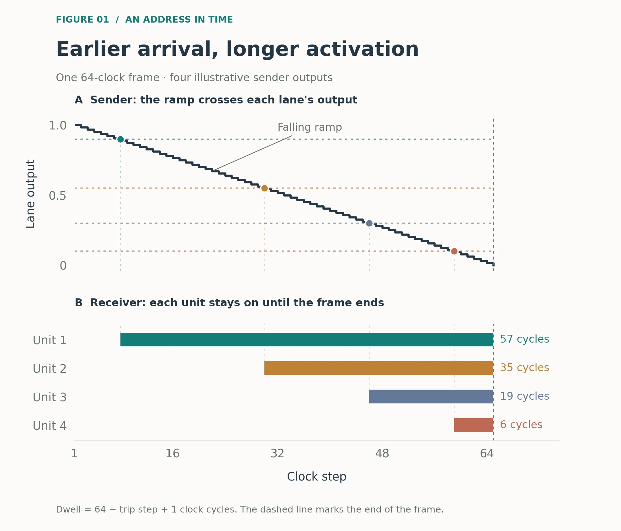
The receiver turns the sender’s trip time into an enabled duration, or dwell. When an address arrives, the receiver enables the corresponding unit and leaves it enabled until the frame ends. If the sender’s lane tripped at step of a -step frame, the receiver unit stays on for
clock cycles. For a linear ramp, this duration is proportional to , the lane’s output above threshold, with negative values set to zero. A receiving lane integrates current from every enabled unit, accumulating charge
where and are the two memristor conductances that form a signed synapse, and is their difference. This is the weighted sum a floating-point layer computes, with activation magnitude represented by duration. At the end of the frame, the receiving bank is read once by its ordinary rank cut. The next bank receives an AAT as before.
The sender does nothing new. It uses the existing ramp, comparators and arbiter, and still sends a digital sequence of addresses. The receiver now uses each address’s arrival time as well as the address itself.
Timing codes have a long history#
The receiver’s enable signals use a familiar code: pulse-width modulation. A December 1945 article in Wireless World describes pulses whose start time varies with signal amplitude while their end time stays fixed. Larger amplitudes start the pulse earlier and make it longer. The dwell receiver uses the same timing convention.
Amplitude-to-time conversion also has a long history in measurement. Wilkinson’s 1950 pulse-amplitude analyser is a classic example. In a Wilkinson ADC, the input pulse charges a capacitor to its peak voltage. A constant current then discharges the capacitor, and counting clock cycles during that discharge measures the original amplitude.
Neural computing has its own timing codes. Hopfield (1995) described a model that represents analog values by the times at which neurons emit action potentials. In neuromorphic hardware, Boahen (2000) describes address-event communication between chips: digital packets identify the neuron that spiked, and their timing conveys when it spiked. A digital address bus can carry both kinds of information.
Time-domain matrix multipliers provide an even closer circuit precedent. Bavandpour, Mahmoodi and Strukov (2019) encode inputs as pulse durations and weights as programmable currents. Integrating those currents onto a capacitor computes the weighted sum. Their output pulses also end at a shared frame boundary. Sahay and colleagues (2020) analyze the same general approach using resistive memory arrays with a transistor selecting each device.
This chapter applies these established ideas to kT-RAM’s rank cut, AAT addressing and local write rule. The experiments test whether its existing address timing can drive a dwell receiver, and whether the public single-pulse rule can teach that receiver.
What the receiver needs#
The feed-forward block requires activation magnitude. What is the smallest change that lets the receiver use it?
The rank cut, sender’s ramp and arbiter, address map, WTA Groups, digital bus, memristor pair per synapse, and write rule all stay the same. The sender can be a bank trained exactly as in Chapter 8.
The receiver needs three additions:
- An enable latch per unit. It is set when the unit’s address arrives and cleared at the end of the frame.
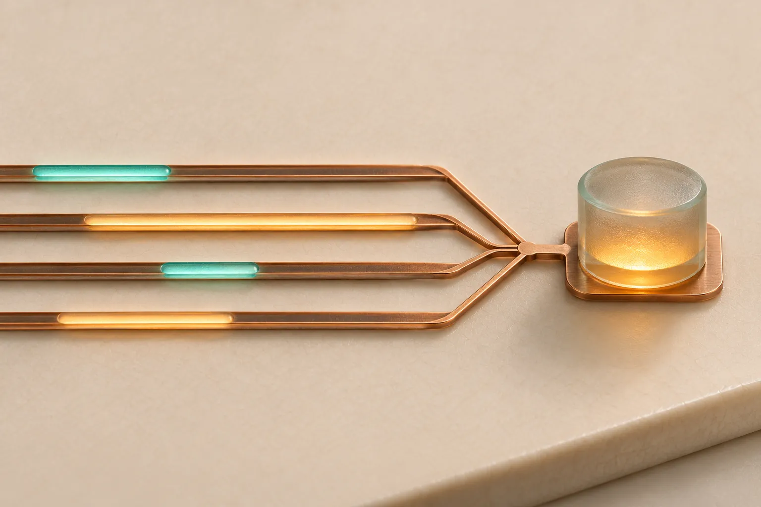
- A current integrator for each lane. A transconductance amplifier supplies the current needed to hold the lane’s node at zero volts. That current is integrated onto a capacitor. Each enabled unit stays at the read voltage for its entire dwell, which may last tens of clock cycles.
- One read at frame end. The bank’s normal rank cut reads the capacitor voltage. The receiver’s gain is : read voltage times clock period, divided by capacitance. A gain shared by all lanes leaves their ranking unchanged in the absence of noise.
Two conventions are also needed. First, the sender’s threshold is zero, so a lane that does not fire contributes nothing. A sweep through both positive and negative values would activate every line on every frame, and the write rule fails under that condition. Signed values therefore use two lines per dimension: one for the positive part and one for the negative part, as in a pair of ReLU activations. Second, banks that do not run in lockstep need a timing record. We store the addresses in trip order with the interval between consecutive trips, , and replay them later using one down-counter. As we will see, four bits per interval are enough.
The same AAT read two ways#
A crossbar’s decoder selects one device pair per read. The receiver therefore cannot activate several symbols in one AAT space at once.
In the codec view from Chapter 7, an AAT is a point in : address spaces, with one of symbols selected in each. An entry specifies a symbol and its space. In the timing view, an entry is the address of a unit crossbar, and the index inside that crossbar selects the layer the lane is emulating. Sender lane maps to receiver unit crossbar . The layer index stays fixed throughout the read and selects the synapses for the neuron being emulated. Changing that index lets one physical lane serve different neurons at different times. The entry’s arrival time determines when its unit turns on.
The AAT uses the same tuple, bits and bus. In emulator terms, the receiver is a bank where is the sender’s lane count and is the number of layers stored in the array. Every active entry in a read selects the same symbol: the current layer index. Each receiving lane integrates current from every enabled unit for that unit’s dwell.
The addresses identify the active inputs, and their arrival times encode the activation magnitudes. The rank cut already provides both; the receiver now uses both.
What the emulator says#
The experiments below used the public emulator with an added dwell-read path. Noise is enabled on both the sender and receiver. Device noise uses the same temperature as the assimilation experiments; comparator noise is 200 µV on a 50 mV read. At each ramp step, we draw a fresh noise sample and record the first step at which each comparator trips. This models a strobed comparator. All experiments use one random seed.
Timing resolution and its limits#
On the stage-1 to stage-2 pair from Chapter 8, the full-resolution dwell code reproduces with of 0.998 at 16 ramp steps and 0.9998 at 64. We also compare the winner in each slot, using the receiver’s own comparator. At , the dwell code agrees with the floating-point target 99.5% of the time. Applied directly to the floating-point outputs, the same noisy comparator selects the correct winner 99.7% of the time. The timing code is within 0.2 percentage points of that noisy floating-point reference.
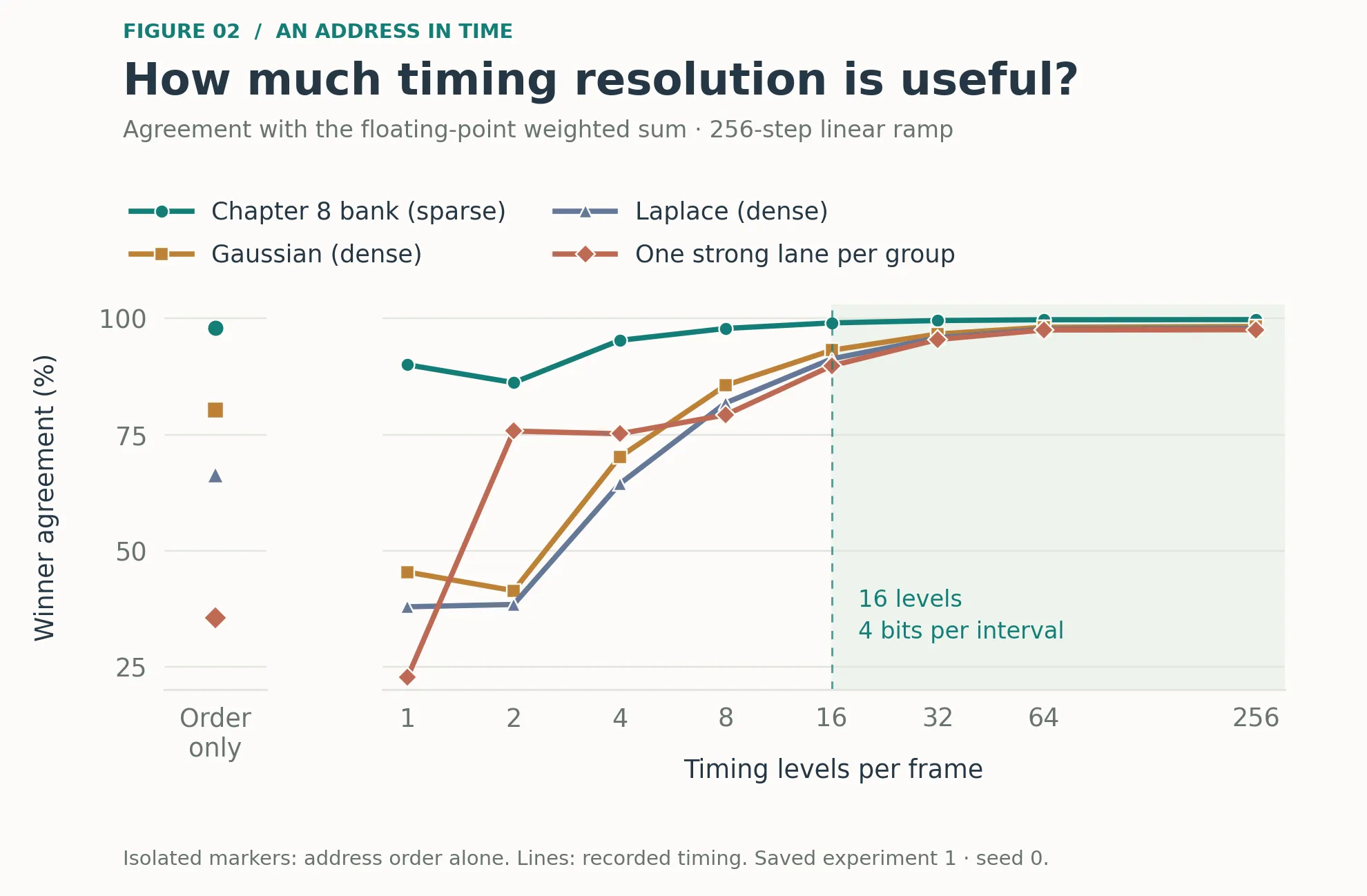
Read noise limits useful timing resolution. The error in estimating from the trip step stops improving near 128 ramp steps. That leaves about 80 distinguishable levels, or six to seven bits of useful timing information. Four bits capture most of the benefit; beyond roughly six bits, extra resolution adds little. Noise also tends to trip lanes slightly early, an effect called first-passage bias. At , that bias is 0.012 steps and is shared by all lanes. The bias is small because noise is likely to cause a crossing only during the few steps when the ramp is close to the lane’s output.
These tests also settled two design choices. A geometric ramp computes a logarithmic sum, , rather than the linear sum required by the teacher. A divider that averages the active lines at each step performs worse than charge integration on every tested input source. We therefore use a linear ramp and integrate the total current.
Signal swing must be large enough for the comparator#
A rank cut depends on relative outputs, so changing the gain over a 64-fold range leaves the noise-free result unchanged. With noise enabled, gain matters: the comparator’s noise stays fixed at 200 µV, so smaller signals are harder to distinguish.
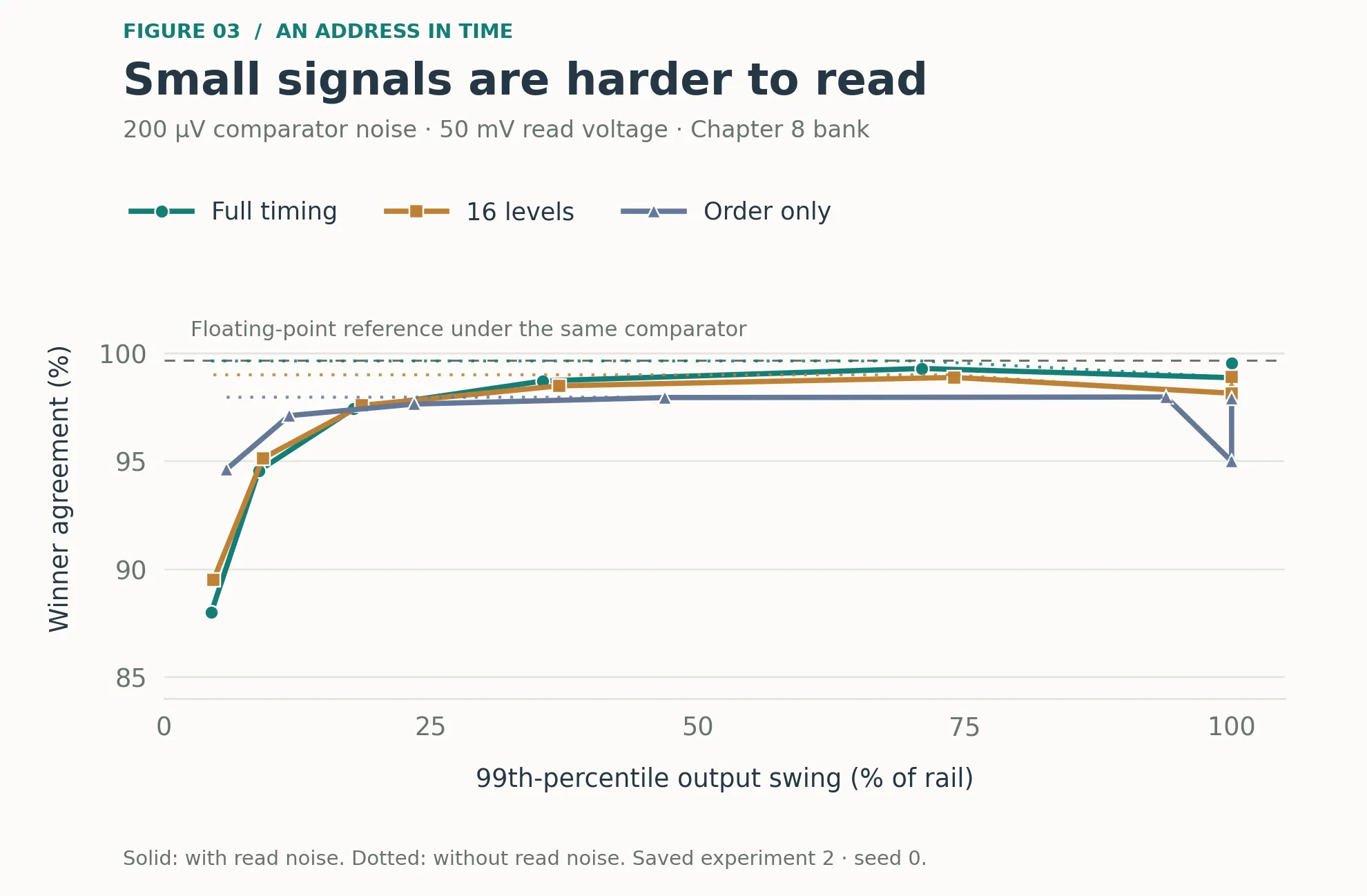
The design rule is to choose the capacitance or clock period so the strongest lane outputs just reach clipping. In these tests, leakage of 1% per clock cycle is tolerable, while 3% is not. The delay between the frame’s end and the receiver’s read accounts for half the time available for leakage, so the receiver should sweep as soon as the frame ends. Among the factors tested, variation in capacitance between lanes is the only one that reduces agreement even without read noise. Teaching the receiver with that variation present largely compensates for it: ±30% variation during teaching reduces agreement by just 0.002.
One write pulse per active line is enough#
The public write rule can teach a receiver that reads dwell input. A fresh stage-2 bank taught from the stage-1 bank’s ramp output reaches 0.845 agreement and 0.849 end-to-end accuracy, matching Chapter 8’s one-hot chain. In that task, however, the identities of the active inputs largely determine the answer. It therefore cannot tell us whether the receiver learned to use their magnitudes.
To test magnitude learning, we used 64 Gaussian input dimensions, all active on every frame and represented on 128 lines to encode sign. A fixed random linear teacher produces outputs in 16 WTA Groups of 16 lanes each, and the target is the winner in each group. The identities of the active inputs provide almost no information about those winners. With dwell reads, the lane bank initially reached only 0.37 agreement, compared with a floating-point ceiling of 0.94. The read carried magnitude, but learning fell far short of that reference.
The write rule applies one pulse per active line whether that line was enabled for two clock cycles or sixty. Scaling the write duration with dwell made learning worse. It also requires additional hardware behavior. The memristor changes state only above its write threshold, so the read dwell does not itself cause an update. A dwell-proportional write requires replaying the frame at a higher voltage, holding each unit on for its dwell. We tested that replay in the byte model and the time-integrating MSS and RS device models. It performed worse at every batch size. At full timing resolution, it drove every synapse to its minimum state in one pass.
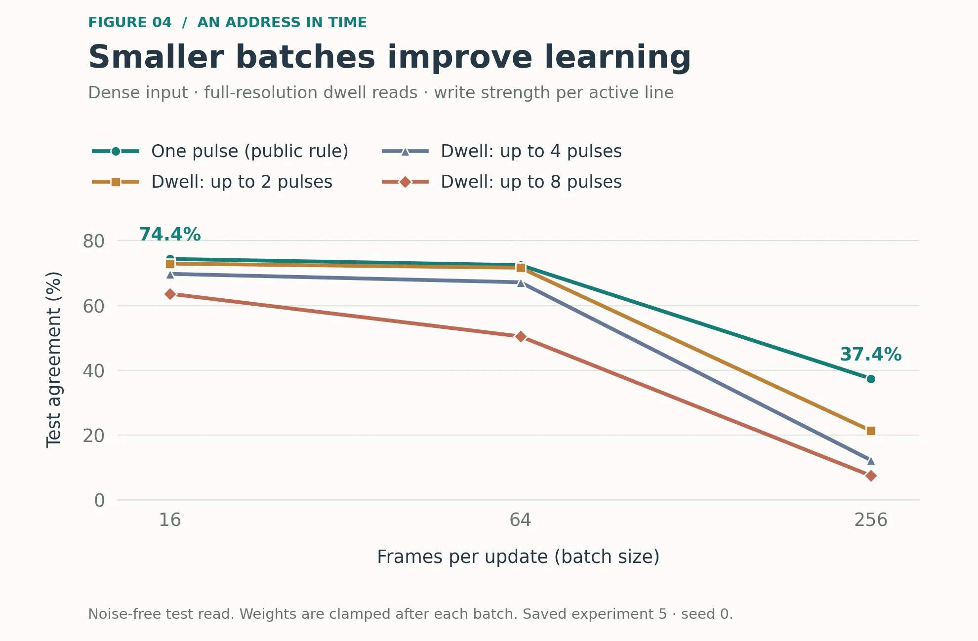
The appropriate floating-point comparison is a perceptron that reads with and updates with . It reaches 0.886 agreement on this task, compared with 0.902 when the update uses and 0.938 with Adam. For the perceptron, omitting magnitude from the update therefore costs little, provided the read still uses it. The lane bank reaches 0.75 with one pulse per active line. Its remaining gap to 0.89 involves the public adapt rule at small batch sizes: the byte step size, decay applied to the fifteen losing lanes per group on every frame, and the ten-epoch training schedule. The experiments did not vary those factors systematically.
Sparsity#
That task used dense input. To test sparse input, we kept only the top of the 64 inputs active in each frame. We scaled the receiver’s gain by to keep the output swing at the rail.
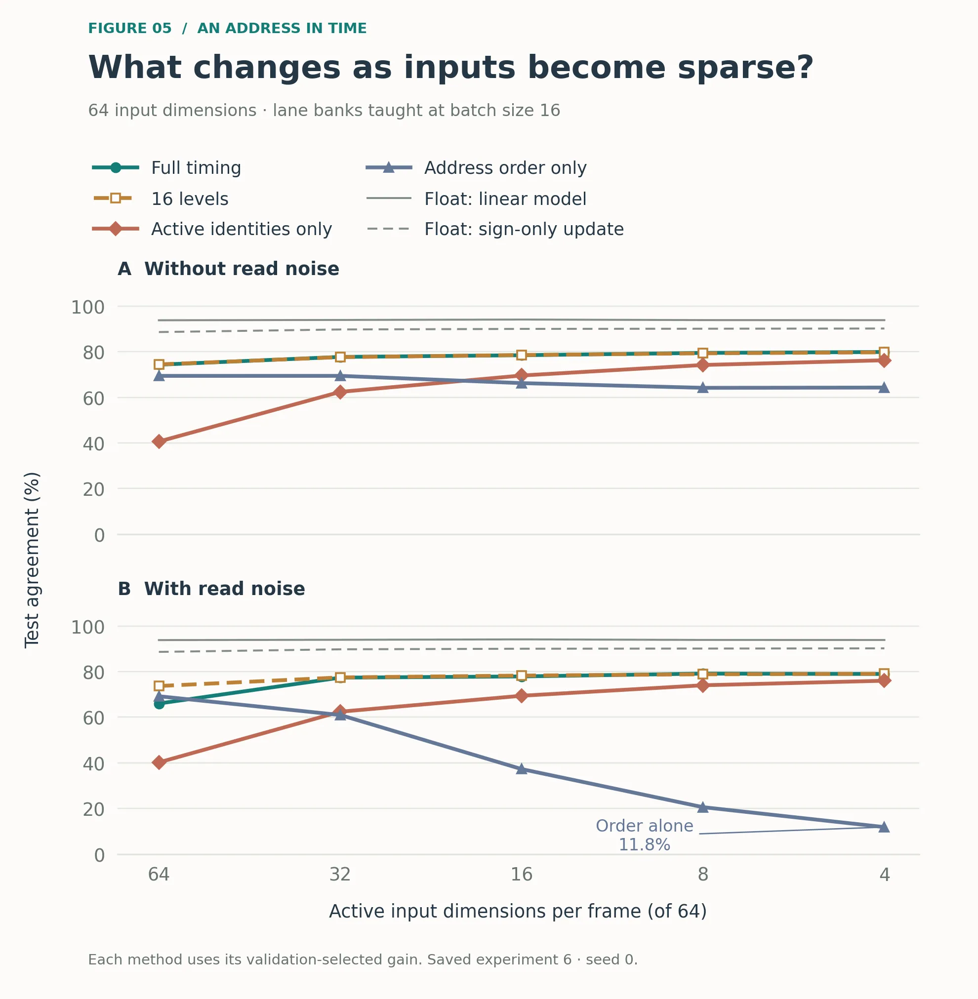
The sparsity tests show three effects.
Sparser input improves learning. The bank’s agreement rises as falls, while the perceptron reference stays fixed. The adapt rule learns more effectively when fewer synapses are updated per frame. Sparsity also reduces the batch-update artifact: at 32 active inputs or fewer, results at batch sizes 256 and 16 differ by no more than 0.03. At 16 active inputs or fewer, they differ by no more than 0.005.
Magnitude contributes less as input becomes sparser, but it still helps. At four active inputs, their identities alone give 0.76 agreement; adding timing raises it to 0.80. A feed-forward projection into a residual stream needs the weighted sums themselves. Agreement on group winners does not measure the accuracy of those values.
Address order alone is too vulnerable to comparator noise on sparse input. Timing can be passed live between banks running in lockstep, or stored as a four-bit record for banks that run at different times. In the live form, the sender’s ramp-step signal clocks the receiver’s latches.
A kT-RAM bank’s address timing carries activation magnitude. Converting that timing into dwell lets the receiver compute weighted sums while keeping the existing sender and digital address bus. The emulator results show that the standard single-pulse write rule can learn from dwell inputs, and that sparsity improves learning. The experiments used one random seed, and the receiver remains unverified on physical hardware.