
kt-ram · neural-lanes · assimilation · aat-codec · knowledge-distillation · local-learning
Chapter 8: Assimilation of an MLP
We train an image classifier to teach a network of kT-RAM neural lanes. We learn its AAT interfaces, measure the input encoder's contribution, and assimilate that encoder as well.
By Alex Nugent ·
Contents
TL;DR#
- A trained MLP can teach a network of kT-RAM neural lanes. The replacement learns from AAT examples and acquires its synapses through the lanes’ local learning rule.
- Learning the AAT interfaces improves transfer. In the initial experiment, accuracy rose from 78.60% with fitted codes to 85.40% with learned interfaces, using the same 657,920 synapses.
- The input encoder supplies most of the useful representation. A taught head directly on the digital encoder reached 84.65% accuracy, versus 86.20% for the full chain, averaged over three seeds.
- The encoder can also be assimilated into lanes. The resulting chain reached 84.81% accuracy across three seeds, 1.39 percentage points below the digital-encoder chain.
- The lane-encoder chain uses zero digital multiply-accumulate operations at inference. Pixel quantization, lane reads, AAT Symbol selection and control still require work.
- These experiments demonstrate assimilation in an emulator. Hardware robustness, energy, area and speed must be evaluated on the physical kT-RAM substrate.
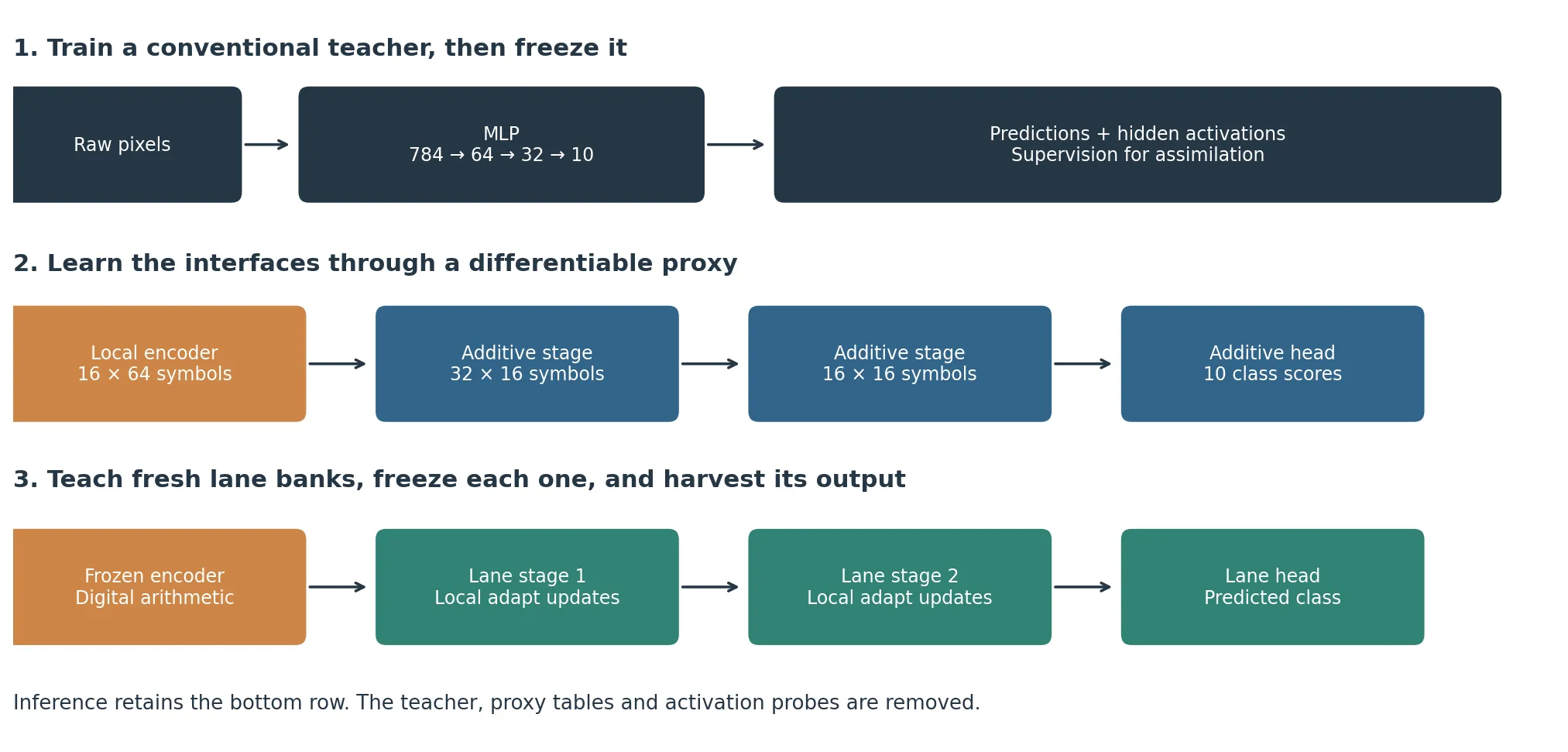
The last three chapters developed ways to represent vectors as Activation Address Tuples, or AATs, choose their codebooks, and perform arithmetic on their symbols. We now use those tools to teach a network of kT-RAM neural lanes from a trained multilayer perceptron, or MLP. The MLP recognizes clothing images; after training, we freeze its parameters and use its behavior to teach a replacement that receives and produces AATs.
This is ASSIMILAATE: Analog Synaptic Systems Implementing Memristor-Integrated Learning and Activation Address Tuple Encoding. The source network supplies AAT examples, while the receiving network acquires its synaptic state through the lanes’ local learning rule.
Learning in situ makes the hardware itself learn the transformation. Feedback uses each lane’s measured response to adjust its conductances, allowing learning to compensate for hardware imperfections, including memristor variation and persistent circuit offsets that affect the teaching readout. The teacher supplies the desired behavior; the hardware develops its own conductance state. Learning can also improve tolerance to random read noise by widening decision margins, reducing how often noise changes an answer without removing the physical noise.
The choice of symbols matters. In the initial experiment, fitting codes to the teacher’s hidden activations produced a taught network with 78.60% accuracy. Learning the interfaces through a differentiable approximation of the receiving network raised that to 85.40%, with the same 657,920 synapses, compared with 88.05% for the frozen teacher. This replacement still used a learned digital network to encode pixels as AATs, so we measured the encoder’s contribution and then assimilated it into lanes as well. All results come from the software emulator.
Teacher Model#
We use Fashion-MNIST, a dataset of 28-by-28 grayscale images in ten clothing categories. The teacher’s dimensions are:
Its computation is
The largest logit in determines the predicted class. The model has 52,650 parameters, including biases, stored in 210,600 bytes at float32, and performs 52,544 multiply-accumulate operations (MACs) per image. We train it on pixels and class labels, then freeze its parameters and record its predicted class and pre-ReLU activations, and , for each training image.
The replacement learns from these records, including the teacher’s mistakes, without using the training labels directly. We measure both accuracy against the dataset labels and agreement with the teacher’s predictions. Learning from another network is established practice in knowledge distillation; here, the receiving stages must also be teachable through the kT-RAM neural lanes’ instructions.
Student Architecture#
An AAT is a tuple with one AAT Symbol in each position, or slot. Each slot has an alphabet of possible symbols; the selected symbol chooses one of that slot’s input channels. The symbol’s numerical value has no ordering significance for the lane. To encode an image, we divide it into sixteen nonoverlapping 7-by-7 patches. A digital 49 → 32 → 64 encoder at each position chooses one AAT Symbol for its patch, producing a 16-slot AAT with one symbol selected from 64 possibilities in each slot. Each encoder sees only its patch, leaving the downstream stages to combine information across the image.
The first stage emits 32 symbols, each from an alphabet of 16. The second emits sixteen symbols, again from alphabets of 16. The head chooses one of ten classes:
Here means slots with possible symbols each, one active per slot. For each output slot, one lane per candidate AAT Symbol receives the input AAT, and the highest-scoring lane determines the emitted AAT Symbol. This winner selection supplies the nonlinearity between stages. In the differentiable proxy, a candidate’s score is a sum of table entries selected by the input symbols:
The input AAT Symbol selects a table entry, while and identify an output slot and candidate AAT Symbol. We train this proxy in PyTorch using one-hot inputs and a linear map. The emulator instead sums the selected differential conductances and divides by their summed magnitudes:
The proxy omits the lane’s changing denominator, finite conductance range and update dynamics. Its accuracy provides a reference for the architecture with AAT interfaces, but neither guarantees nor bounds the taught chain’s accuracy. We must measure that chain separately.
AAT Interfaces#
We compare fitted and learned AAT interfaces using the same architecture and synapse count:
| Configuration | Hidden AAT targets | Digital input encoder |
|---|---|---|
| Fitted interfaces | Produced by codecs fitted to the teacher’s activations. | Trained to predict the first-layer codes, then frozen. |
| Learned interfaces | Learned through the differentiable proxy. | Starts from the fitted configuration and continues training with the proxy. |
For the fitted interfaces, we fit AAT codecs to the teacher’s training activations, and . Each slot encodes two coordinates by selecting one of sixteen possible symbols, so the 64-dimensional first activation becomes 32 symbols, and the 32-dimensional second activation becomes sixteen. Each AAT Symbol refers to a reconstruction value in a fitted codebook. We train the input encoder through an additive reader that predicts the first-layer codes, then freeze the encoder and teach the lane stages these fitted targets. The taught chain reached 78.60% accuracy.
At inference, each hidden stage passes symbols directly to the next without decoding them into vectors, so reconstruction is an indirect objective for this classifier. We can instead choose symbols for their usefulness to the receiving stages. For the learned interfaces, the proxy learns the hidden AATs at the same slot counts and alphabet sizes, while the input encoder continues training from the fitted configuration. Three additive stages connect the encoder to the output, with a discrete AAT Symbol choice in each slot.
We train through these choices with a straight-through estimator: the forward pass chooses an AAT Symbol in one-hot form, while the backward pass follows a softmax approximation. Three terms guide learning: classification against the teacher’s predictions, reconstruction of and through linear probes, and a usage-entropy bonus that encourages use of the full alphabet. Probe errors are normalized by the variance of the teacher activations.
The probes encourage the codes to retain information about the teacher’s activations. Their outputs never feed the next stage, and the probes are removed after training. The learned proxy with discrete AATs reached 85.75% accuracy; we then tested whether the local rule could acquire its behavior.
Local Teaching Procedure#
We freeze the proxy, record its codes for the training images, and teach fresh lane banks through Classifier.adapt. For an output slot with possible symbols, candidate occupies lane , so the target AAT selects one lane per output slot:
target_lanes = target_codes + alphabet * torch.arange(output_slots)bank.adapt(input_codes, target_lanes, feedback="hard")The library performs an adapting FF read, then applies RH to targets, RL to non-targets that fired, and RF otherwise. These instructions set the conductances; no optimizer or copied proxy table sets them. We teach the stages in order:
- Teach the first bank from input-encoder codes to the proxy’s first hidden codes. Freeze it and record its actual outputs.
- Teach the second bank from those actual first-bank outputs to the proxy’s second hidden codes. Freeze it and record its actual outputs.
- Teach the head from the actual second-bank outputs to the original teacher’s predicted classes.
If the first bank emits AAT Symbol 7 where the proxy emitted 3, the second bank must learn from 7 because that is what it will receive at inference. Its target remains the proxy’s second-stage code for the image. On hardware, teaching from actual outputs lets downstream stages adapt to persistent upstream device errors and comparator offsets, provided those outputs are collected under the intended inference conditions. This adaptation still depends on the information preserved upstream: if an earlier stage gives identical codes to inputs requiring different answers, later stages cannot distinguish them.
In batched adapt, examples share readings taken before the update. A batch of 256 is therefore different from 256 serial updates. The companion allows either procedure.
Assimilation Results#
The taught chain with learned interfaces reached 85.40% accuracy, 0.35 percentage points below its proxy, with 89.85% teacher agreement. It exceeded the chain with fitted interfaces by 6.80 percentage points at the same synapse count.
The comparison involved several changes: refining the input encoder, learning new hidden targets, changing the objective, and doubling the first bank’s teaching epochs. A companion run with equal teaching budgets reproduced the improvement: 78.90% with fitted interfaces and 84.90% with learned interfaces, against an 88.35% teacher. Both runs used the historical 2,000-image evaluation set, which was repeatedly inspected during development. They demonstrate transfer, but leave the digital encoder’s contribution unresolved.
Input Encoder Contribution#
The sixteen patch MLPs contain 59,392 parameters and perform 57,856 MACs per image, exceeding the teacher’s entire network at 52,544. Each sees only one patch, yet their outputs may already support most of the classification. To measure the hidden stages’ contribution, we compared encoders with the downstream hidden interfaces fixed at 32×16 and 16×16. For each encoder, we also taught a fresh ten-lane head directly on its frozen output. Comparing this head-only control with the full chain shows how much accuracy the two hidden stages add.
The encoder study used a custom split of the pooled dataset: 32,000 training images, 2,000 validation images and a 36,000-image test set, including the historical 2,000. Validation selected checkpoints before test evaluation. The main comparisons used three initialization seeds with the split and frozen teacher fixed. These test results are reported separately from the historical results above.
With the digital patch MLP, the head alone reached 84.65%, compared with 86.20% for the full chain, averaged over three seeds. The two hidden stages added about 1.6 percentage points, showing that the encoder’s symbols already support most of the achieved accuracy. The encoder was learned with the full proxy, however, so this control does not show that head-only training would learn an equally useful encoder.
Input Encoder Assimilation#
To replace the digital encoder with lanes, we quantize each pixel to four levels: one represents the zero background, and the others divide nonzero training pixels by quantiles. The thresholds are shared across positions and fixed before teaching. Each patch becomes a 49-slot AAT, with one slot for each pixel position. Each slot contains one AAT Symbol identifying that pixel’s quantized level, chosen from four possible symbols. A group of 64 lanes reads this AAT and emits the winning lane’s AAT Symbol; sixteen groups produce the same 16×64 interface as the digital encoder.
We learn the patch symbols with the downstream proxy, then teach them to a fresh grouped bank through Classifier.adapt. We freeze that bank and teach the downstream stages on its actual outputs. All four stages acquire their synapses through the local rule.
The chain reached 84.81 ± 0.15%, compared with 86.20 ± 0.22% for the digital-encoder chain, a loss of 1.39 percentage points. These are means and initialization standard deviations over three seeds. The head-only control shows a similar contribution from the hidden stages:
| Frozen encoder | Encoder + taught head | Encoder + full taught chain |
|---|---|---|
| Digital patch MLP, 64 symbols | 84.65% | 86.20% |
| Taught lane encoder, 64 symbols | 83.42% | 84.81% |
Both rows average three seeds, and a single taught head comes within about 1.5 points of either full chain. In the second row, the encoder supplying those symbols is itself a taught lane stage.
The lane-encoder chain uses zero digital MACs at inference. Four-level pixel quantization still requires 1,568 comparisons per image, counted at two per pixel, with lane reads, AAT Symbol selection and control adding further work.
Synapses and Computation#
Replacing the digital encoder adds synapses. A lane stage with input slots, channels per slot, and output candidates requires
The encoder has synapses, and the downstream banks add 657,920, giving 858,624 synapses in total. To explore the tradeoffs in synapse count and digital arithmetic, we also tested linear digital encoders and patch alphabets of 16 symbols. Smaller alphabets reduce the first downstream bank’s size while leaving the hidden interfaces fixed.
| Input encoder | Test accuracy | Seeds | Digital MACs/image | Total synapses | Software payload, kB |
|---|---|---|---|---|---|
| Patch MLP, 64 symbols | 86.20 ± 0.22% | 3 | 57,856 | 657,920 | 1,553 |
| Linear, 64 symbols | 85.55 ± 0.49% | 3 | 50,176 | 657,920 | 1,521 |
| Linear, 16 symbols | 85.12% | 1 | 12,544 | 264,704 | 581 |
| Taught lanes, 64 symbols | 84.81 ± 0.15% | 3 | 0 | 858,624 | 1,717 |
| Taught lanes, 16 symbols | 83.56 ± 0.06% | 3 | 0 | 314,880 | 630 |
The ± values are initialization standard deviations. Software payload counts four bytes per float32 parameter and two per packed synapse, including the lane encoders’ three float32 thresholds. One kB is 1,000 bytes. Both lane encoders use the same pixel-quantization comparisons; lane work is additional to the digital MAC column.
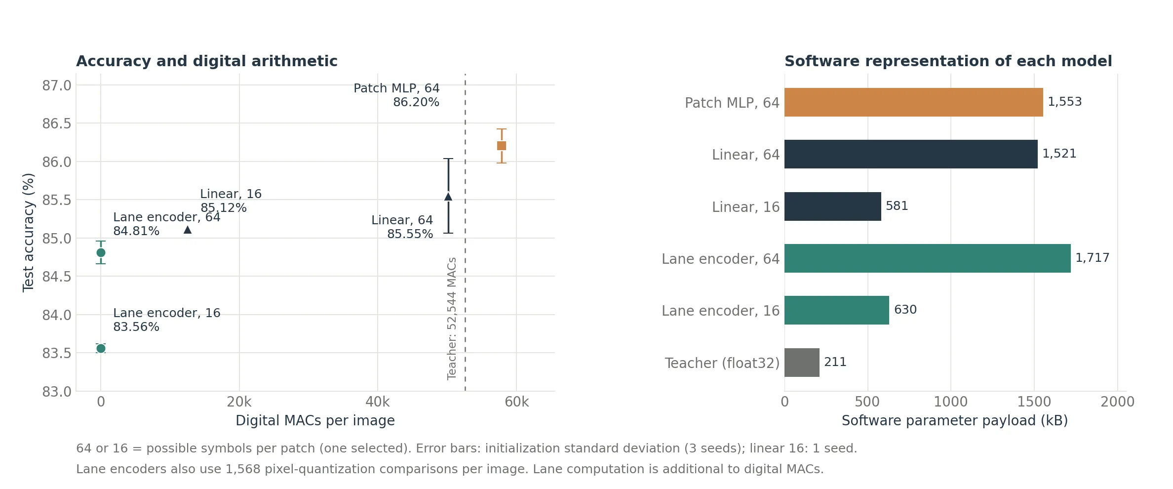
The byte counts describe the chosen software representation. On physical kT-RAM, synaptic state resides in device conductances, and storage density depends on the devices and circuitry used to realize the lanes. Hardware robustness, energy, area and speed require measurements on that substrate. Accuracy here was measured on live emulator banks, whose conductance buffers alone use eight bytes per synapse. The packed payload counts exclude metadata, activations and runtime overhead, and quantized exports need separate accuracy measurements.
The per-seed experiment record contains the test and control results, proxy validation results, split hashes and exact cost counts.
Teaching Limitations#
Proxy validation accuracy was similar for the lane encoder and digital MLP: 86.30% and 86.40%. Yet the taught encoder with 64 possible symbols per patch matched only about 65% of its proxy’s patch symbols, making acquisition of the encoder’s function a bottleneck. AAT Symbol agreement is a diagnostic, however: increasing it does not necessarily improve classification.
At batch size 256, frequently active background synapses received many updates from the same earlier reading, and encoder agreement oscillated between epochs. Reducing the encoder batch to 64 improved acquisition. All lane-encoder results above use this setting; downstream teaching stays at batch 256 with 20/10/10 epochs. The remaining gap is a teaching limitation under this procedure, with longer teaching and serial updates still untested.
Hardware compensation requires the teaching loop to observe the errors present at inference. A different read path or voltage can change those errors. The planned comparator-offset and noise experiments for this MLP chain remain to be done.
Companion Implementation#
The companion in python/examples/mlp-assimilation/ in the ktram-neural-core checkout runs the original fitted-versus-learned comparison, saves reloadable students and checks packed exports.
python -m pip install -e './python[torch,examples]' 'scikit-learn>=1.2'python python/examples/mlp-assimilation/experiment.py --smokepython python/examples/mlp-assimilation/experiment.pyThe smoke run uses scikit-learn’s bundled digits dataset, while the full run uses Fashion-MNIST, validation-based checkpoint selection and equal teaching budgets. Add --freeze-input to hold the input encoder fixed during interface learning. The encoder study uses encoder_screen.py and encoder_teach.py in the same folder, with the full run’s frozen teacher; the companion README lists the commands.
Scaling to Larger Models#
LUT-NN and Differentiable Weightless Neural Networks provide precedents for learning representations and functions for lookup-based inference. Assimilation adds a local acquisition step: fresh lane banks must learn the functions defined by those interfaces.
This MLP demonstrates that process from quantized pixels to class prediction. The encoder supplies much of the useful representation, and teaching it is a substantial part of the transfer problem. A separate shared convolutional experiment produced a larger transfer gap, so depth, weight sharing and other tasks need further study.
In a transformer, query and key AATs used by attention need a numerical interpretation. Outputs entering the residual stream must reconstruct compatible values. Hidden AATs inside an assimilated feed-forward block may have more freedom, as they do here. SwiGLU, attention and repeated residual updates still need transfer experiments.
The procedure is the same: freeze the source, learn interfaces for the receiving network, teach each stage on its predecessor’s actual outputs, and evaluate the complete replacement, including the input encoder. On physical kT-RAM, the goal is to acquire that transformation in the presence of the devices’ own variations, offsets and noise.