Chapter 7c: Attention on AATs

Chapter 7 called computing on AATs the codec’s second job. Chapter 7b made the first job practical: Codec G brought the reconstruction tables down to a few hundred bytes, and Codec N replaced exhaustive centroid search with scalar bin assignments. Those small tables store reconstruction values, not every product an attention score might need. The remaining question is how to do the arithmetic from the symbols.

The kT-RAM neural lanes consume and produce AATs. To connect them to a transformer, we also need the operations between its matrix transforms: attention scores, weighted value sums, normalization, and residual addition. Here we work out the score and the value blend, which reuse one codebook across many tokens.

Kernel costs#

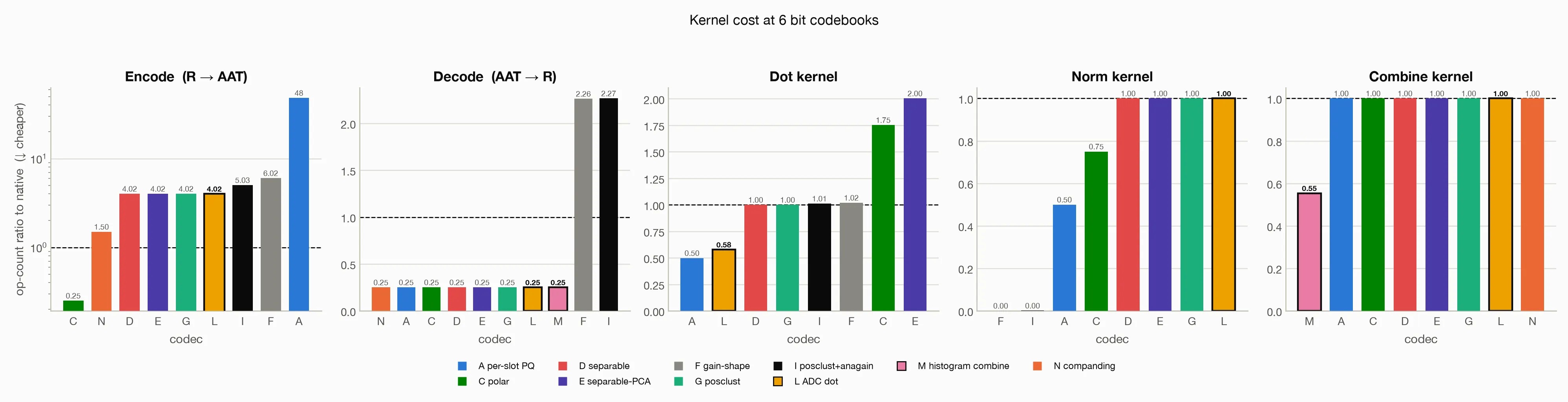
We use Chapter 7b’s operation-count model: a table lookup, a multiply, and an add each count as one. A dot product on 128 floats uses 128 multiplies and 127 adds, or 255 operations; a kernel costing half as much scores 0.5×. The ratios include each kernel’s setup but exclude encoding, decoding, and surrounding operations such as softmax. They are operation counts, not timings or energy measurements.

The fidelity experiments use held-out activations In machine learning, these are examples kept separate while fitting the codebook. They show whether it also works on data it has not seen. from a middle layer of Qwen3-0.6B, as in Chapter 7b. At the six-bit working point, each 128-number attention vector becomes 64 two-number slots, a point in $\mathbb{A}_{64}^{64}$. The norm experiment uses 1,024-number residual-stream vectors; the image example uses Fashion-MNIST separately.

Codec L and Codec M retain G’s fitted codebooks and change how the symbols are read: L computes inner products, and M computes weighted value sums. Query, key, and value vectors can each have their own fitted books.

The attention score in AAT space#

The raw attention score is an inner product In vector math, multiply the query and key at each matching position, then add the products. The result is one signed number. , $\text{score} = \langle \hat{q}, \hat{k} \rangle$, where the hats denote decoded approximations of a query and a key. Attention scales these scores by $1/\sqrt{D}$, applies the causal mask, and uses softmax In a transformer, the mask hides future positions. Softmax turns the remaining scores into nonnegative weights that add up to one. to obtain the weights for the value blend. Here we count only the inner product.

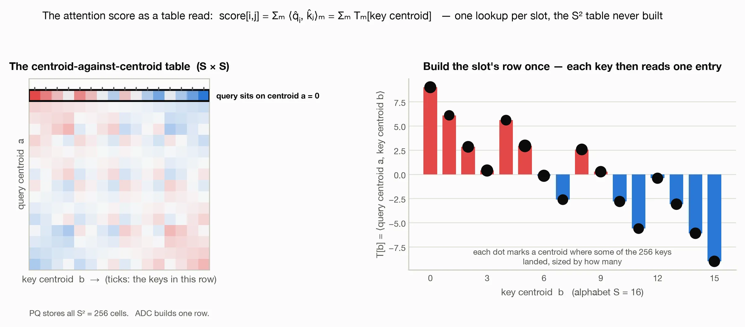
Because the code is built slot by slot, the dot product splits into a sum over 64 slots. Let $C_m^Q$ and $C_m^K$ be the query and key codebooks at slot $m$. For query $i$ and key $j$, the symbols $a_{im}$ and $b_{jm}$ select the two centroids:

$$\begin{aligned} \text{score}[i,j] \;=\; \langle \hat{q}_i, \hat{k}_j \rangle \;&=\; \sum_{m} \bigl\langle\, C_m^Q[a_{im}],\; C_m^K[b_{jm}] \,\bigr\rangle \\[4pt] &=\; \sum_{m} G_m[\, a_{im},\, b_{jm} \,]. \end{aligned}$$

$G_m[a,b] = \langle C_m^Q[a], C_m^K[b] \rangle$ is the contribution of centroid pair $(a,b)$. Storing every pair would make scoring cheap but, as Chapter 7b showed, per-slot books and product tables take about 540 KB. Codec G stores only scalar reconstruction values and calculates their products, at a modeled dot-product cost near 1.0× native.

One query is scored against a whole row of keys, so the query holds still while the keys stream past. At each slot it needs only one row of the square table, $G_m[a_{im},\cdot\,]$. Build just that row: $T_m[b] = G_m[a_{im},b]$, with $S$ entries instead of $S^2$. Each key then costs one lookup per slot, and the full score is $\sum_m T_m[b_{jm}]$. The row-building work is shared across every key that query scores.

This is Codec L, the ADC dot, borrowing the search literature’s term asymmetric distance computation. It sums the same centroid products as Codec G, so the change preserves the signed inner product, including its magnitude.

Separability also reduces the row-building work. For an 8-by-8 grid, multiply the query’s two coordinates by the eight levels on their respective axes, then add the resulting pairs to form the 64 entries. Across 64 slots, the rows need 8 KiB of temporary storage at two bytes per entry, in addition to the compact codebooks.

This row lookup follows product-quantization search, including FAISS. Conventional ADC keeps the query unquantized; here the query can itself be an AAT.

The value blend as a histogram#

Attention’s output is a weighted average of value vectors, $z = \sum_j \alpha_j v_j$, where $\alpha_j$ are the softmax weights. Averaging symbol indices has no numerical meaning: the mean of indices 12 and 50 does not identify the mean of their centroids. We can, however, accumulate weights by symbol and read the resulting totals against the codebook.

In one slot, every value vector contributes a single centroid: value $j$ decodes to $C[c_j]$, one of the $S$ centroids in that slot’s book. So the slot’s output is $\sum_j \alpha_j C[c_j]$, a weighted sum over the $T$ values. Now regroup that same sum by centroid instead of by value:

$$\begin{aligned} z[m] \;&=\; \sum_{j} \alpha_j \, C[c_j] \\[4pt] &=\; \sum_{c} \Bigl(\, \sum_{j \,:\, c_j = c} \alpha_j \Bigr)\, C[c] \\[4pt] &=\; \sum_{c} w[c] \, C[c]. \end{aligned}$$

$w[c]$ is the total attention weight assigned to centroid $c$. Each slot needs its own histogram, even when slots share a codebook. Codec M scatters the $T$ weights into those bins, costing $T$ additions per slot, then reads the histogram against the centroid values. For two-number centroids, the readout performs a weighted sum for each of the two coordinates. Its work scales with the alphabet size $S$, while each incoming value contributes only its symbol index.

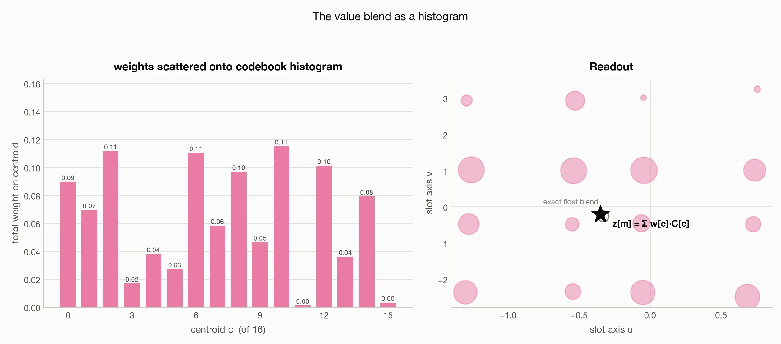
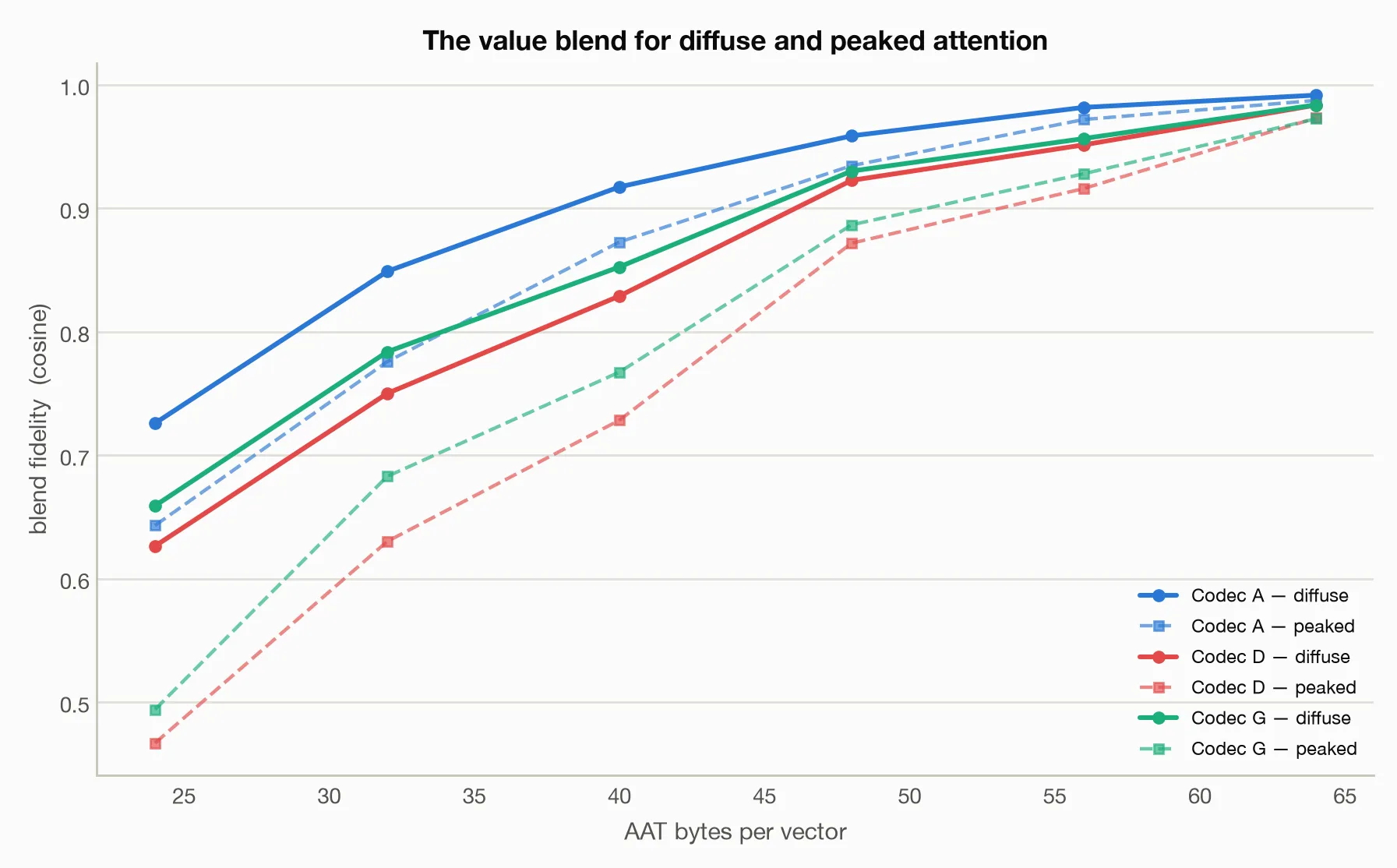
For fixed weights, regrouping gives the same blend as decoding every value first, up to numerical rounding. The six-bit experiment reports 0.908 cosine From vector geometry: a cosine similarity of 1 means two vectors point in the same direction; 0 means they are at right angles. It does not compare their lengths. against the blend of the original values. Because it holds the weights fixed, that result isolates value-coding error; it does not measure a full attention block with coded scores.

At 256 values, Codec M’s modeled cost is 0.554× native, using the cheaper of the two histogram layouts described below. Its flat histogram needs 16 KiB of temporary storage with 32-bit accumulators, in addition to the value codebook.

The output $z$ is a real-valued vector. If the next lane expects symbols, that output still needs encoding. The saving is that the kernel avoids reconstructing all $T$ input value vectors.

Longer context, lower op cost#

Codec L builds its lookup rows once per query, then reads them for every key. Codec M accumulates weights for every value, then reads out the histogram once. Longer rows spread that fixed work over more tokens.

Codec L’s read is 64 lookups and 63 adds, one per slot, while the score it returns costs 128 multiplies and 127 adds in floats: 127 operations against 255, so the score floors at half of native.

Codec M does one add per slot per value: value $j$‘s weight goes into the bin for its centroid, 64 slots, 64 adds, no multiply. In floats that same value contributes a multiply and an add on each of its 128 elements, 256 operations. So the blend floors at a quarter of native. Reading the histogram back is the fixed part, one pass over the alphabet per slot, and it does not grow with the row.

The blend has two histogram layouts. The flat tally accumulates one weight per value over all 64 centroids. The split tally uses the separable grid: in the illustrated 8-by-8 case, it accumulates weights into two eight-bin histograms and reads out each axis separately. That reduces the readout work but doubles the accumulation, since every value updates a bin on both axes. The cost model selects the split tally for short rows and the flat tally for long ones, with a crossover near 270 keys in this configuration. Only the flat tally approaches a quarter of native cost.

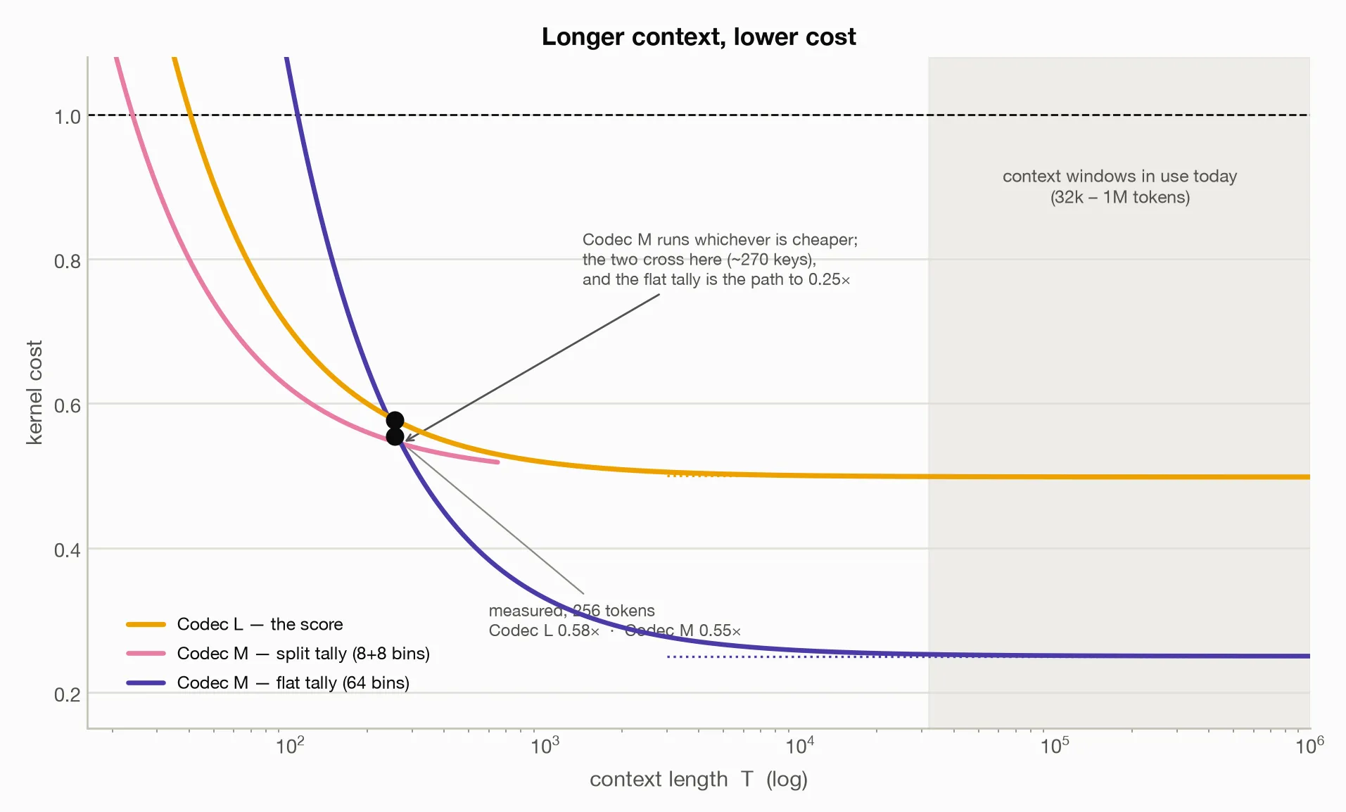
These kernels reduce the cost of each score and blend; dense attention still takes $O(T^2)$ work over a full sequence. The plotted ratios apply to a row of the given length, not to the average row in a causal pass, whose early positions see fewer keys.

The norm#

The norm is a vector’s length. Codec G calculates it from the selected scalar values, with a modeled cost near native arithmetic. At six bits, the residual-stream experiment in $\mathbb{R}^{1024}$ reports 0.949 correlation with the original norms. As Chapter 7b noted, correlation alone does not measure magnitude error.

The near-zero bars in the scorecard belong to gain-shape codecs, which store a vector’s length separately from its direction. Recovering length is then a read, but reconstruction multiplies the selected direction by the selected gain. That product requires an extra operation beyond a lane’s additive readout, so this family was set aside for the current design.

Bit ops#

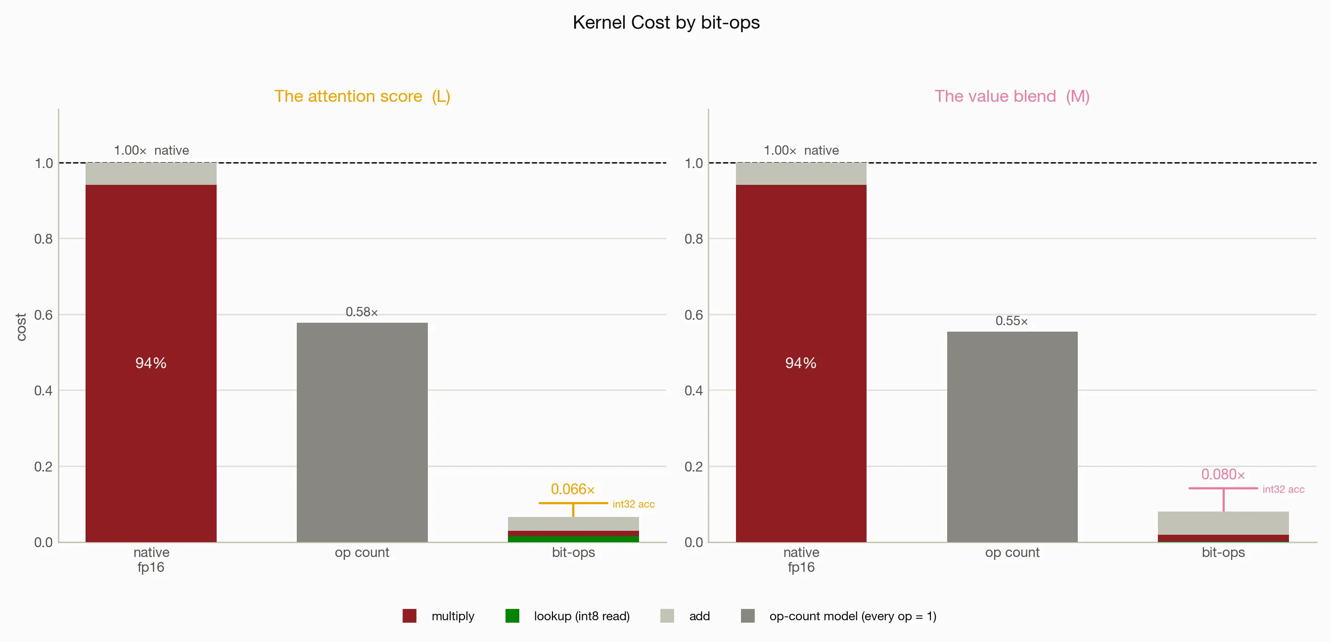
The first scorecard counts every operation equally. A second model, bit-ops, weights a multiply by the product of its operand widths, an add by its accumulator width In digital arithmetic, the accumulator holds a running sum. A wider one can hold a larger total before overflow. , and a lookup by the word read. A nominal 16-by-16 multiply thus counts as 256, a 16-bit add as 16, and an int8 lookup as eight. This simplified model does not predict elapsed time or energy.

Under those assumptions, multiplication contributes about 94% of the native fp16 dot-product budget. Codec L replaces per-key products with lookups, while Codec M replaces per-value products with histogram additions; multiplication remains in the fixed setup or readout. Their modeled costs are about 0.07× and 0.08× the native baseline, or 0.10× and 0.14× with 32-bit kernel accumulators. Int8 lookup entries introduce quantization error that the fidelity measurements above do not cover.

The KV cache#

In autoregressive generation, a transformer retains previous keys and values in its KV cache and reads them for each new token. A 128-number vector stored as 64 packed six-bit symbols occupies 48 bytes, compared with 256 bytes in fp16: 5.3× less vector payload. The current PyTorch reference uses integer-index tensors, so 48 bytes describes a packed format, not its measured cache size.

Codec L can score the cached symbols and Codec M can blend them without reconstructing every key or value. That combination offers narrower storage and computation, provided a runtime implements the packed layout and the symbol reads efficiently.

Whole images from sums of codewords#

Chapter 7 introduced an additive image codec that lets every symbol contribute to the entire output, rather than to one fixed pair of coordinates. It uses the same lookup-and-sum operation:

$$\hat{x} = \mu + \sum_{m=1}^{M} A_m[c_m].$$

For a 28×28 Fashion-MNIST image, $A_m[c_m]$ selects a 784-number contribution, or atom, from book $m$; $\mu$ is the stored mean image. This is additive quantization. With 128 books of 16 atoms, the code uses 512 bits per image and reaches 0.0500 relative MSE, versus 0.0576 for a patch-codec reference at the same bit budget. Relative MSE divides reconstruction error by the source pixel variance; lower is better.

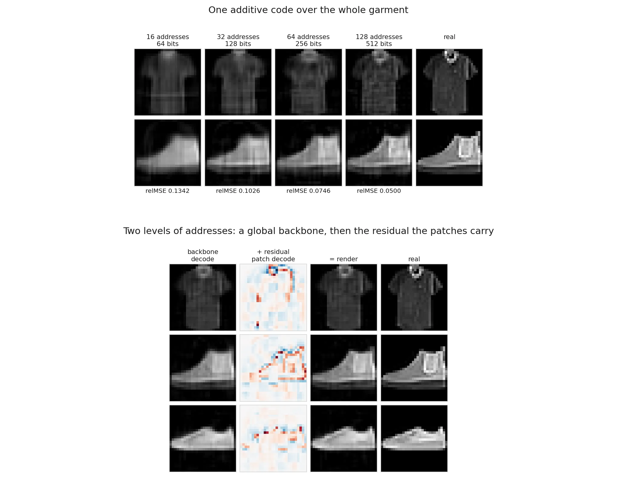
CHILL ZEN generates images in that 904-bit global-plus-patch code. It samples the symbols on neural lanes and turns them into pixels with this additive decoder. Its companion paper proposes an in-memory implementation of the decoder and includes it in the energy budget.

Whole-image atoms require much larger shared codebooks than Chapter 7b’s scalar tables, so these image results are separate from the attention-kernel cost comparison.

The resulting interface#

Codec G’s compact books can be read in two new ways: L builds query-specific rows for attention scores, and M groups value weights by symbol. Both reduce modeled operation counts without changing what the fitted symbols mean. The AAT codec module provides the reference implementation; testing the packed format and complete-model behavior is the next step.